26. Turbulence, Earnings Instability, and Indirect Inference#
26.1. Overview#
Ljungqvist and Sargent [1998] and Ljungqvist and Sargent [2008] attribute the persistently high unemployment in Europe after 1980 to an interaction between unemployment benefits tied to past earnings and an increase in what they call economic turbulence, the risk of losing skills when a job ends in a layoff.
To check whether an increase in turbulence is consistent with evidence about earnings in the United States, Ljungqvist and Sargent [1998] generated artificial panels of earnings from the laissez-faire version of their model at two levels of turbulence.
They applied to those panels the decomposition of earnings into permanent and transitory components that Gottschalk and Moffitt [1994] had applied to men in the Panel Study of Income Dynamics (PSID) for 1970–78 and 1979–87, and they compared the resulting histograms with Gottschalk and Moffitt’s.
Ljungqvist and Sargent [2008] repeated the check in a richer model, with turbulence parameters \(0.1\) and \(0.2\) for the two windows.
Ljungqvist and Sargent [1998] concluded that “an increase in our turbulence parameter spreads the distributions of both components of the Gottschalk-Moffitt decomposition in the direction observed.” They added:
It is also noteworthy that the increased earnings variability in the more turbulent period in our figure 14b occurs at lower standard deviations than in Gottschalk and Moffitt’s findings. In this respect, the increase in economic turbulence in our parameterization of the 1980s falls short of the changes documented for the United States.
In this lecture we describe their check as a comparison of information projections and make it quantitative for the model of Ljungqvist and Sargent [1998].
Gottschalk and Moffitt’s decomposition is the m-projection, in the sense of Information Projections, of the distribution of a man’s nine annual log earnings in a balanced panel onto a Gaussian random-effects model.
Ljungqvist and Sargent’s check compares the data’s histograms of men’s averages and standard deviations with their model’s at two values of the turbulence parameter; the second moments of those histograms are the parameters of the projections. Computing the model’s projection at every value of that parameter gives what Gourieroux et al. [1993] call the binding function, and choosing the parameter to make the two projections agree is the method of indirect inference that Which Moments to Match? describes.
With the 1970–78 turbulence parameter held at Ljungqvist and Sargent’s value of \(0.02\), no value of the 1979–87 parameter lets the laissez-faire model deliver more than about one fifth of the increase in the permanent variance that Gottschalk and Moffitt measured, or more than about 45 percent of the increase in the transitory variance. With both parameters free, the bounds are about one third and one half.
These bounds depend on the range of skills and on the speed of skill transitions. Doubling the range alone lets turbulence deliver about 46 percent of the increase in the permanent variance and nearly all of the increase in the transitory variance; doubling the transition probabilities as well brings the permanent share back to about one fifth.
An increase in the layoff rate moves Gottschalk and Moffitt’s two statistics in the same direction as an increase in turbulence, and in a sample of Gottschalk and Moffitt’s size the two statistics barely distinguish the two explanations.
The covariance-structure model of Moffitt and Gottschalk [2011], a second auxiliary model, attributes the earnings instability that turbulence creates almost entirely to a transitory component, while Gottschalk and Moffitt’s decomposition attributes about half of it to the permanent component.
The lecture proceeds as follows.
Laissez-faire economy describes the laissez-faire economy of Ljungqvist and Sargent [1998] and reproduces their steady-state statistics.
Gottschalk and Moffitt’s decomposition describes Gottschalk and Moffitt’s decomposition as an information projection.
Ljungqvist and Sargent’s check reproduces Ljungqvist and Sargent’s check and computes the binding function.
Layoff rates and turbulence compares turbulence with a higher layoff rate.
Covariance-structure model describes a second auxiliary model.
The lecture builds on Information Projections, Which Moments to Match?, and Specification Tests.
Job Search I: The McCall Search Model and Job Search II: Search and Separation describe simpler search models.
We use the following imports.
import numpy as np
import matplotlib.pyplot as plt
from collections import namedtuple
from scipy.stats import norm, chi2, ncx2
from scipy.optimize import minimize
26.2. Laissez-faire economy#
26.2.1. Workers#
Ljungqvist and Sargent [1998] study a continuum of risk-neutral workers.
A period is two weeks.
Each worker dies with probability \(\alpha\) between periods and maximizes \(E_t \sum_{i=0}^\infty \beta^i (1 - \alpha)^i y_{t+i}\), where \(y_t\) is income net of the disutility of searching.
A newborn worker starts unemployed with the lowest skill level.
A worker’s skill \(h\) takes one of 21 values evenly spaced on \([1, 2]\).
An employed worker earns \(w h\), where \(w\) is the wage per unit of skill on the job.
At the beginning of each period, an employed worker is laid off with probability \(\lambda\).
A worker who is not laid off gains one skill level with probability \(0.1\) and keeps the wage \(w\) until a layoff, a quit, or death.
The skill of an unemployed worker falls by one level with probability \(0.2\) each period, and the lowest level is absorbing.
An unemployed worker chooses a search intensity \(s \in [0, 1]\) at a disutility \(c(s) = 0.5 s\), and receives one wage offer next period with probability \(\pi(s) = s^{0.3}\).
Wage offers are drawn from a normal distribution with mean \(0.5\) and variance \(0.1\), truncated to \([0, 1]\).
Ljungqvist and Sargent define turbulence as follows:
Economic turbulence is defined in terms of the mean and variance of skill losses associated with layoffs. We now let the skills of a newly laid-off worker be distributed according to the left half of a normal distribution, with the range starting at the lowest possible skill level and ending at the worker’s skill level before the layoff.
They obtain the distribution by taking the left half of a normal distribution centered on \(0.5\) and confined to \([0, 1]\), stretching it over the skill levels from the lowest to the level that the worker held before the layoff, and normalizing it.
The variance of that normal distribution indexes turbulence; we call it the turbulence parameter.
When the turbulence parameter is zero, a laid-off worker keeps the skill level held before the layoff.
Let \(\mu_e(h, h')\), \(\mu_u(h, h')\), and \(\mu_l(h, h')\) be the skill transition probabilities of an employed worker, an unemployed worker, and a worker who has just been laid off.
The laissez-faire economy has no unemployment benefits and no taxes.
The value \(V(w, h)\) of a worker with skill \(h\) who holds or is offered a job with wage \(w\), and the value \(V_u(h)\) of an unemployed worker, satisfy
and
The second argument of the max in \(V(w, h)\) is the option to reject the offer or to quit.
Let \(G(h) = (1 - \alpha)\beta \sum_{h'} \mu_u(h, h') [\int V(w, h') \, dF(w) - V_u(h')]\) be the expected gain from an offer.
The first-order condition for search intensity gives \(s(h) = \min\{1, (0.6 \, G(h))^{1/0.7}\}\).
In the laissez-faire economy the bound binds, and \(s(h) = 1\) at every skill level, as Ljungqvist and Sargent report.
Ljungqvist and Sargent set \(\beta = 0.9985\), an annual interest rate of 4 percent, \(\alpha = 0.0009\), an expected working life of 42.7 years, and \(\lambda = 0.009\), an expected 4.3 years of employment before a layoff.
26.2.2. Computation#
The function create_model stores the primitives.
Its arguments h_max, up, and down set the range of skills and the probabilities of skill gains and losses, which we change in an exercise.
Model = namedtuple("Model", ("β", "α", "λ", "turbulence", "h_grid", "w_grid",
                             "f_w", "μ_e", "μ_u", "μ_l"))


def layoff_matrix(n_h, turbulence):
    """Skill transitions at a layoff: the left half of a normal distribution
    centered on 0.5, stretched over the skill levels up to the current one."""
    μ_l = np.eye(n_h)
    if turbulence > 0:
        for j in range(1, n_h):
            x = 0.5 * np.arange(j + 1) / j
            weights = np.exp(-(x - 0.5)**2 / (2 * turbulence))
            μ_l[j] = 0.0
            μ_l[j, :j + 1] = weights / weights.sum()
    return μ_l


def create_model(turbulence=0.0, β=0.9985, α=0.0009, λ=0.009,
                 h_max=2.0, up=0.1, down=0.2, n_h=21, n_w=101):
    h_grid = np.linspace(1, h_max, n_h)
    w_grid = np.linspace(0, 1, n_w)
    pdf = norm.pdf(w_grid, 0.5, np.sqrt(0.1))
    μ_e = np.eye(n_h) * (1 - up)
    μ_e[np.arange(n_h - 1), np.arange(1, n_h)] = up
    μ_e[-1, -1] = 1.0
    μ_u = np.eye(n_h) * (1 - down)
    μ_u[np.arange(1, n_h), np.arange(n_h - 1)] = down
    μ_u[0, 0] = 1.0
    return Model(β, α, λ, turbulence, h_grid, w_grid, pdf / pdf.sum(),
                 μ_e, μ_u, layoff_matrix(n_h, turbulence))
The figure shows the distribution of skills after a layoff for a worker who had the highest skill level, for the two values of the turbulence parameter that Ljungqvist and Sargent use to represent 1970–78 and 1979–87.
fig, ax = plt.subplots()
for v in (0.02, 0.04):
    m = create_model(turbulence=v)
    ax.plot(m.h_grid, m.μ_l[-1], "o-", label=f"turbulence parameter {v}")
ax.set_xlabel("skill after the layoff")
ax.set_ylabel("probability")
ax.legend()
plt.show()
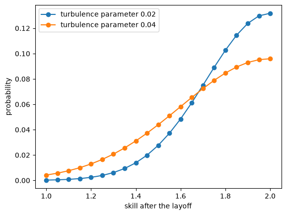
Fig. 26.1 Skill after a layoff from the top level#
We solve the Bellman equations by value iteration and return the acceptance decisions and search intensities.
def solve_model(m, tol=1e-9, max_iter=100_000):
    δ = (1 - m.α) * m.β
    earnings = np.outer(m.w_grid, m.h_grid)
    V = np.zeros_like(earnings)
    V_u = np.zeros(len(m.h_grid))
    for _ in range(max_iter):
        W = earnings + δ * ((1 - m.λ) * V @ m.μ_e.T
                            + m.λ * (m.μ_l @ V_u)[None, :])
        V_new = np.maximum(W, V_u[None, :])
        gain = δ * m.μ_u @ (m.f_w @ V - V_u)
        s = np.clip((0.6 * np.maximum(gain, 0))**(1 / 0.7), 0, 1)
        V_u_new = -0.5 * s + δ * m.μ_u @ V_u + s**0.3 * gain
        error = max(np.abs(V_new - V).max(), np.abs(V_u_new - V_u).max())
        V, V_u = V_new, V_u_new
        if error < tol:
            break
    accept = W >= V_u[None, :]          # accept[w, h]
    return accept, s
The next function computes the stationary distribution of workers across employment states, wages, and skills, with newborn workers replacing those who die.
From it we compute the unemployment rate, the average duration of unemployment, and the average earnings of employed workers, which Ljungqvist and Sargent call average productivity.
def steady_state(m, accept, s, tol=1e-12, max_iter=200_000):
    n_w, n_h = len(m.w_grid), len(m.h_grid)
    E, U = np.zeros((n_w, n_h)), np.zeros(n_h)
    U[0] = 1.0
    survive = 1 - m.α
    for _ in range(max_iter):
        E_kept = survive * (1 - m.λ) * E @ m.μ_e
        quits = np.where(accept, 0.0, E_kept).sum(axis=0)
        laid_off = survive * m.λ * E.sum(axis=0) @ m.μ_l
        offers = survive * (U * s**0.3) @ m.μ_u
        hires = np.outer(m.f_w, offers) * accept
        E_new = np.where(accept, E_kept, 0.0) + hires
        U_new = survive * U @ m.μ_u - hires.sum(axis=0) + quits + laid_off
        U_new[0] += m.α
        error = np.abs(E_new - E).max() + np.abs(U_new - U).max()
        E, U = E_new, U_new
        if error < tol:
            break
    inflow = quits.sum() + laid_off.sum() + m.α
    earnings = np.outer(m.w_grid, m.h_grid)
    return {"unemployment rate": U.sum(),
            "duration (weeks)": 2 * U.sum() / inflow,
            "average productivity": (E * earnings).sum() / E.sum()}
Table 5 of Ljungqvist and Sargent [1998] reports these statistics for the laissez-faire economy at four values of the turbulence parameter: unemployment rates of 6.28, 5.81, 5.77, and 5.73 percent; average durations of 11.8, 10.6, 10.6, and 10.7 weeks; and average productivities of 1.659, 1.552, 1.520, and 1.496.
print("turbulence   unemployment   duration   productivity   search intensity")
for v in (0.0, 0.02, 0.03, 0.04):
    m = create_model(turbulence=v)
    accept, s = solve_model(m)
    stats = steady_state(m, accept, s)
    print(f"{v:9.2f} {100 * stats['unemployment rate']:12.2f}% "
          f"{stats['duration (weeks)']:10.1f} {stats['average productivity']:13.3f}"
          f"        {s.min():.2f} to {s.max():.2f}")
turbulence   unemployment   duration   productivity   search intensity
     0.00         6.36%       11.9         1.657        1.00 to 1.00
     0.02         5.92%       10.8         1.552        1.00 to 1.00
     0.03         5.84%       10.7         1.521        1.00 to 1.00
     0.04         5.82%       10.8         1.498        1.00 to 1.00
Our computations agree with their table to within 0.11 percentage points of unemployment, 0.2 weeks of duration, and 0.002 units of productivity, and search intensity equals one at every skill level.
In the laissez-faire economy, turbulence lowers productivity, because laid-off workers lose skills, and it barely changes unemployment.
The welfare state of Ljungqvist and Sargent [1998], in which benefits are tied to past earnings, responds very differently: its unemployment rate rises from 6.95 to 14.87 percent as the turbulence parameter rises from 0 to 0.04.
26.2.3. Artificial panels#
Ljungqvist and Sargent [1998] describe how they generated their panels:
For the laissez-faire economy, we generated artificial panels of length 9 years with 10,000 individuals for two different subperiods: relatively tranquil economic times and more turbulent times as indexed in table 5 by variances .02 and .04, respectively. The former panel is meant to represent the period 1970–78 in the Gottschalk-Moffitt study, and the latter panel would then correspond to the period 1979–87. For both panels, we use as initial conditions the equilibrium distribution of workers who have been in the labor force for 20 years.
We draw such initial conditions by simulating newborn workers for 20 years, conditional on their survival.
The function below records two-week earnings, employment, layoffs, and skills.
def draw_next(cum_rows, rows, u):
    """Draw the next state for each worker from rows of cumulative probabilities."""
    return (u[:, None] > cum_rows[rows]).sum(axis=1)


def simulate_workers(m, accept, s, N, T, T_burn, seed=0):
    rng = np.random.default_rng(seed)
    cum_e, cum_u, cum_l = (np.cumsum(μ, axis=1) for μ in (m.μ_e, m.μ_u, m.μ_l))
    cum_w = np.cumsum(m.f_w)
    n_w = len(m.w_grid)
    emp, wi, hj = np.zeros(N, bool), np.zeros(N, int), np.zeros(N, int)
    record = {"earn": np.zeros((N, T)), "emp": np.zeros((N, T), bool),
              "laid": np.zeros((N, T), bool), "h": np.zeros((N, T), int)}
    for t in range(T_burn + T):
        u = rng.random((N, 4))
        new_emp, new_wi, new_hj = emp.copy(), wi.copy(), hj.copy()
        laid = emp & (u[:, 0] < m.λ)
        kept = emp & ~laid
        new_hj[laid] = draw_next(cum_l, hj[laid], u[laid, 1])
        new_emp[laid] = False
        new_hj[kept] = draw_next(cum_e, hj[kept], u[kept, 1])
        new_emp[kept & ~accept[wi, new_hj]] = False          # quits
        idle = ~emp
        new_hj[idle] = draw_next(cum_u, hj[idle], u[idle, 1])
        offer = np.minimum((u[:, 2][:, None] > cum_w).sum(axis=1), n_w - 1)
        hired = idle & (u[:, 3] < s[hj]**0.3) & accept[offer, new_hj]
        new_emp[hired], new_wi[hired] = True, offer[hired]
        emp, wi, hj = new_emp, new_wi, new_hj
        if t >= T_burn:
            k = t - T_burn
            record["earn"][:, k] = np.where(emp, m.w_grid[wi] * m.h_grid[hj], 0.0)
            record["emp"][:, k], record["laid"][:, k], record["h"][:, k] = emp, laid, hj
    return record


def log_annual_earnings(record, years=9):
    """Log annual earnings with year means removed, for workers with
    positive earnings in every year."""
    annual = record["earn"].reshape(len(record["earn"]), years, 26).sum(axis=2)
    positive = (annual > 0).all(axis=1)
    y = np.log(annual[positive])
    return y - y.mean(axis=0), positive.mean()


def artificial_panel(turbulence, N=10_000, seed=0, **kwargs):
    m = create_model(turbulence=turbulence, **kwargs)
    record = simulate_workers(m, *solve_model(m), N=N, T=9 * 26,
                              T_burn=20 * 26, seed=seed)
    return log_annual_earnings(record)
Gottschalk and Moffitt removed a common age profile from log earnings before decomposing them.
All workers in an artificial panel have the same experience, so we remove only the mean of log earnings in each year.
A worker who is unemployed for a whole year has no log earnings, and we drop such workers, about a quarter of one percent of the panel.
26.3. Gottschalk and Moffitt’s decomposition#
26.3.1. Definitions#
Gottschalk and Moffitt [1994] study white men in the PSID who were aged 20 to 59, were household heads and not students, and had positive wage and salary earnings.
They trim the top and bottom 1 percent of the earnings distribution within age-education-year cells.
They regress log real annual earnings on a quartic in age, separately for 1970–78 and 1979–87, and decompose the residuals \(y_{it}\) of man \(i\) in year \(t\) as \(y_{it} = \mu_i + \nu_{it}\).
They take as the permanent component of man \(i\) the average \(\bar y_i\) of \(y_{it}\) over the \(T_i\) years in which the man appears in a window, and as the transitory component the deviations \(y_{it} - \bar y_i\).
Their appendix gives the formulas
where \(\bar y\) is the mean of \(y_{it}\) over all men and years and \(\bar T\) is the average of \(T_i\).
The transitory variance \(\sigma^2_\nu\) is the average of the men’s own variances of earnings around their averages.
The permanent variance \(\sigma^2_\mu\) is the variance of the men’s averages, less the part of that variance that the transitory components contribute.
Their Table 1 reports that the permanent variance rose from \(0.201\) in 1970–78 to \(0.284\) in 1979–87, and that the transitory variance rose from \(0.104\) to \(0.148\).
They write that “fully one-third of the widening of the earnings distribution has resulted from a rise in the instability of earnings.”
The function gm_decomposition computes formulas (26.1), and the function trim drops the top and bottom 1 percent of each year’s log earnings, which makes a panel unbalanced.
gm_data = {"1970-78": np.array([0.201, 0.104]),
           "1979-87": np.array([0.284, 0.148])}
gm_change = gm_data["1979-87"] - gm_data["1970-78"]


def gm_decomposition(y, keep=None):
    """Permanent and transitory variances, formulas (ti_gm); keep marks the
    years in which each man appears."""
    if keep is None:
        keep = np.ones(y.shape, bool)
    T_i = keep.sum(axis=1)
    y_bar_i = np.where(keep, y, 0).sum(axis=1) / T_i
    σ2_ν = (np.where(keep, (y - y_bar_i[:, None])**2, 0).sum(axis=1)
            / (T_i - 1)).mean()
    σ2_μ = ((y_bar_i - y[keep].mean())**2).sum() / (len(y) - 1) - σ2_ν / T_i.mean()
    return np.array([σ2_μ, σ2_ν])


def trim(y, q=0.01):
    """Drop the top and bottom fraction q of each year's log earnings, remove
    the year means again, and keep the men who remain in at least two years."""
    lo, hi = np.quantile(y, [q, 1 - q], axis=0)
    keep = (y >= lo) & (y <= hi)
    y = y - np.where(keep, y, 0).sum(axis=0) / keep.sum(axis=0)
    two_years = keep.sum(axis=1) >= 2
    return y[two_years], keep[two_years]
26.3.2. Decomposition as information projection#
Let \(y_i = (y_{i1}, \ldots, y_{iT})\) be the vector of a man’s log earnings in a window of \(T\) years, and suppose that every man appears in every year of the window, as in a balanced panel.
The random-effects model says that \(y_{it} = m + a_i + e_{it}\), where \(a_i \sim N(0, \sigma^2_\mu)\) and the \(e_{it} \sim N(0, \sigma^2_\nu)\) are independent of each other and over time.
Under this model \(y_i\) is normal with mean \(m \mathbf{1}\) and covariance matrix \(\sigma^2_\mu \mathbf{1}\mathbf{1}^\top + \sigma^2_\nu I\), where \(\mathbf{1}\) is a vector of ones.
The inverse of that covariance matrix is a linear combination of \(I\) and \(\mathbf{1}\mathbf{1}^\top\), so the random-effects model is an exponential family.
Its sufficient statistics are the average \(\bar y_i\), its square \(\bar y_i^2\), and the within sum of squares \(W_i = \sum_t (y_{it} - \bar y_i)^2\).
In the notation of Approximation Errors in Time Series Models, \(T \bar y_i^2\) is the periodogram of a man’s earnings at frequency zero, and by Parseval’s identity \(W_i\) is the sum of the periodogram ordinates at the other \(T - 1\) Fourier frequencies \(2\pi j / T\).
The model’s distribution of earnings is discrete, so its KL divergence from every normal distribution is infinite, as Information Projections notes.
The proof of Theorem 23.2 applies instead to the cross-entropy \(-E[\log q_\theta(y_i)]\), which differs from the KL divergence by the entropy of \(y_i\) whenever \(y_i\) has a density.
For any distribution of \(y_i\) with the same mean in every year and a nonsingular covariance matrix whose average off-diagonal element is nonnegative, the parameters that minimize the cross-entropy match the expectations of the sufficient statistics, which sets \(m = E[\bar y_i]\) and
Solving gives \(\sigma^2_\nu = E[W_i]/(T - 1)\) and \(\sigma^2_\mu = \operatorname{Var}(\bar y_i) - \sigma^2_\nu / T\).
We call this minimizer the m-projection of the distribution of \(y_i\) onto the random-effects model.
The projection sets \(\sigma^2_\nu\) equal to the average expected periodogram at the nonzero Fourier frequencies, and, for \(y_i\) with mean zero, as in our year-demeaned panels, \(T\sigma^2_\mu + \sigma^2_\nu\) equal to the expected periodogram at frequency zero.
For a balanced panel, Gottschalk and Moffitt’s permanent and transitory variances are the parameters of the m-projection of the distribution of a man’s earnings onto the random-effects model: formulas (26.1) are the expressions above with the sample of men in place of the population, apart from the divisor \(N - 1\) in the variance of the averages.
The projection is defined whether or not the random-effects model describes the data.
Gottschalk and Moffitt report correlations of 0.14 and 0.18 between successive transitory components and conclude that the components are “largely uncorrelated.”
Under the random-effects model, the correlation between successive deviations \(y_{it} - \bar y_i\) is \(-1/(T - 1)\), or \(-0.125\) when \(T = 9\).
Gottschalk and Moffitt’s correlations therefore lie about \(0.3\) above what serially uncorrelated transitory components would produce.
The cross-entropy of a normal distribution depends on the distribution of \(y_i\) only through its mean and its covariance matrix \(S\), so we can compute the projection by minimizing the KL divergence of \(N(0, S)\) from the random-effects model.
The projection’s parameters are linear functions of \(S\):
Exercise 26.2 derives these formulas.
So if log earnings are the sum of two independent components, the projection of the sum is the sum of the projections.
The random-effects covariance matrices and their inverses lie in the same linear space, spanned by \(I\) and \(\mathbf{1}\mathbf{1}^\top\).
The sufficient statistics are quadratic forms \(y_i^\top A y_i\) with \(A\) in that space, so matching their expectations makes \(S - \Sigma\) orthogonal to the space in the trace inner product.
Since \(\Sigma\) lies in the space, the m-projection coincides with the least squares projection of \(S\) onto it, which sets \(\sigma^2_\mu\) equal to the average off-diagonal element of \(S\) and \(\sigma^2_\mu + \sigma^2_\nu\) equal to the average diagonal element.
A linear space of covariance matrices does not by itself make the two projections coincide: the symmetric Toeplitz matrices, which include the covariance matrices of stationary processes, form a linear space that does not contain their inverses, and the two projections onto it differ.
The code below checks both characterizations, and the periodogram identities, for an artificial panel.
def random_effects_cov(θ, T=9):
    σ2_μ, σ2_ν = θ
    return σ2_μ * np.ones((T, T)) + σ2_ν * np.eye(T)


def gaussian_kl(S, Σ):
    """KL divergence of N(0, S) from N(0, Σ)."""
    M = np.linalg.solve(Σ, S)
    sign, logdet = np.linalg.slogdet(M)
    return 0.5 * (np.trace(M) - len(S) - logdet) if sign > 0 else np.inf


def euclidean(S, Σ):
    """Sum of squared differences of the distinct elements of S and Σ."""
    upper = np.triu_indices(len(S))
    return np.sum((S[upper] - Σ[upper])**2)


y02, kept = artificial_panel(0.02)
S = np.cov(y02.T)
for name, distance in (("KL", gaussian_kl), ("least squares", euclidean)):
    res = minimize(lambda p: distance(S, random_effects_cov(np.exp(p))),
                   np.log([0.02, 0.05]), method="Nelder-Mead",
                   options={"xatol": 1e-10, "fatol": 1e-14})
    print(f"{name:14} projection: {np.round(np.exp(res.x), 5)}")
print(f"formulas (ti_gm):         {np.round(gm_decomposition(y02), 5)}")
print(f"fraction of workers kept: {kept:.4f}")

T = y02.shape[1]
periodogram = np.abs(np.fft.fft(y02, axis=1))**2 / T
W = ((y02 - y02.mean(axis=1, keepdims=True))**2).sum(axis=1)
print("largest Parseval discrepancies:",
      np.abs(periodogram[:, 0] - T * y02.mean(axis=1)**2).max(),
      np.abs(periodogram[:, 1:].sum(axis=1) - W).max())
KL             projection: [0.01544 0.0489 ]
least squares  projection: [0.01544 0.0489 ]
formulas (ti_gm):         [0.01544 0.04889]
fraction of workers kept: 0.9974
largest Parseval discrepancies: 2.220446049250313e-15 3.552713678800501e-15
For a stationary process with spectral density \(f\), in the convention of Approximation Errors in Time Series Models, the formulas in \(S\) give
where \(K_T(\omega) = \sin^2(T\omega/2) / (T \sin^2(\omega/2))\) is the Fejér kernel, the periodogram at frequency \(\omega\) of a sequence of \(T\) ones; the expected periodogram at frequency zero is \(\frac{1}{2\pi}\int_{-\pi}^{\pi} f(\omega) K_T(\omega) \, d\omega\).
The weight on \(f\) in \(\sigma^2_\mu\) equals one at frequency zero and integrates to zero, so \(\sigma^2_\mu\) measures the excess of the spectral density near frequency zero over its average.
With \(T = 9\), about nine tenths of the Fejér kernel’s weight lies at frequencies \(|\omega| < 2\pi/T\).
Let’s check (26.2) against the formulas in \(S\) for two autoregressions.
n_grid = 2**14
ω = 2 * np.pi * (np.arange(n_grid) + 0.5) / n_grid - np.pi
K = np.sin(T * ω / 2)**2 / (T * np.sin(ω / 2)**2)
for ρ in (0.7, -0.4):
    f = 1 / np.abs(1 - ρ * np.exp(-1j * ω))**2
    lags = np.abs(np.subtract.outer(np.arange(T), np.arange(T)))
    S_ar = ρ**lags / (1 - ρ**2)
    σ2_ν = (np.trace(S_ar) - S_ar.sum() / T) / (T - 1)
    print(f"ρ = {ρ:4}: Fejér form {np.mean(f * (K - 1)) / (T - 1):.6f}, "
          f"{np.mean(f * (T - K)) / (T - 1):.6f};  "
          f"formulas in S {S_ar.sum() / T**2 - σ2_ν / T:.6f}, {σ2_ν:.6f}")
print(f"share of the Fejér kernel's weight at |ω| < 2π/T: "
      f"{np.mean(K * (np.abs(ω) < 2 * np.pi / T)):.3f}")
ρ =  0.7: Fejér form 0.737259, 1.223525;  formulas in S 0.737259, 1.223525
ρ = -0.4: Fejér form -0.078284, 1.268760;  formulas in S -0.078284, 1.268760
share of the Fejér kernel's weight at |ω| < 2π/T: 0.907
For the negatively autocorrelated process the formulas give a negative \(\sigma^2_\mu\), because its spectral density lies below its average near frequency zero; its m-projection onto the random-effects model lies on the boundary \(\sigma^2_\mu = 0\).
The linearity of the projection in \(S\) justifies comparing changes between windows even though the model and the data differ in levels.
The model’s workers are identical when they enter the labor force, and the model has no measurement error, so its permanent and transitory variances are far below Gottschalk and Moffitt’s.
Suppose that the data’s log earnings are the sum of a component that the model describes and an independent component whose covariance matrix is the same in the two windows.
Then the change in the data’s projection from 1970–78 to 1979–87 equals the change in the projection of the component that the model describes.
Hansen and Sargent’s ideal seasonal adjustment in Approximation Errors in Time Series Models follows the same strategy: it compares a model that omits a feature of the data with the data only where the omitted feature drops out.
There the comparison uses the frequencies outside the seasonal bands; here it uses the changes between windows.
Gottschalk and Moffitt’s evidence supports the maintained assumption more for the transitory variance than for the permanent variance.
Measurement error raises their transitory variances, and they write that “the issue is whether this bias has changed over time. We know of no evidence that it has.”
They write that “an increase in the price of ‘skill’ may be a satisfactory explanation for changes in the dispersion of permanent wages,” and Ljungqvist and Sargent’s workers are ex ante identical, so their model has no education or other characteristic fixed at entry whose price could rise.
26.4. Ljungqvist and Sargent’s check#
26.4.1. Histograms#
Ljungqvist and Sargent [1998] use Gottschalk and Moffitt’s evidence “partly to inspire and partly to check our model.”
Their check compares histograms of the men’s averages \(\bar y_i\) and of their standard deviations around those averages.
The figure below plots Gottschalk and Moffitt’s histograms, which we read approximately from their Figures 2 and 4, above the histograms of our artificial panels for the turbulence parameters \(0.02\) and \(0.04\).
y04, _ = artificial_panel(0.04)

gm_fig2_bins = np.arange(-1.75, 1.01, 0.25)
gm_fig2 = {"1970-78": [0.7, 0.4, 1.1, 2.9, 5.6, 11.3, 16.9, 21.5, 23.2, 10.9, 4.1, 1.3],
           "1979-87": [1.1, 1.05, 1.95, 3.05, 6.2, 10.4, 15.1, 19.7, 18.7, 13.95,
                       6.4, 2.0]}
gm_fig4_bins = np.arange(0.1, 1.21, 0.1)
gm_fig4 = {"1970-78": [42.4, 22.8, 12.6, 8.1, 6.05, 2.55, 1.65, 1.15, 1.0, 0.75,
                       0.25, 0.45],
           "1979-87": [36.4, 22.25, 12.75, 7.8, 6.3, 4.45, 3.05, 2.3, 1.4, 0.7,
                       0.9, 1.15]}


def percent_histogram(x, centers):
    width = centers[1] - centers[0]
    edges = np.append(centers - width / 2, centers[-1] + width / 2)
    return 100 * np.histogram(np.clip(x, edges[0], edges[-1] - 1e-9), edges)[0] / len(x)


model_mean_bins = np.arange(-0.5, 0.51, 0.1)
model_sd_bins = np.arange(0.1, 0.71, 0.1)
fig, axes = plt.subplots(2, 2, figsize=(11, 7))
for ax, bins, data, title in ((axes[0, 0], gm_fig2_bins, gm_fig2, "PSID, average"),
                              (axes[0, 1], gm_fig4_bins, gm_fig4,
                               "PSID, standard deviation")):
    width = bins[1] - bins[0]
    ax.bar(bins - width / 5, data["1970-78"], width=0.4 * width, label="1970–78")
    ax.bar(bins + width / 5, data["1979-87"], width=0.4 * width, label="1979–87")
    ax.set_title(title)
    ax.set_ylabel("percent")
    ax.legend()

for ax, bins, stat, title in (
        (axes[1, 0], model_mean_bins, lambda y: y.mean(axis=1), "model, average"),
        (axes[1, 1], model_sd_bins, lambda y: y.std(axis=1, ddof=1),
         "model, standard deviation")):
    width = bins[1] - bins[0]
    for shift, y, label in ((-1, y02, "turbulence 0.02"), (1, y04, "turbulence 0.04")):
        ax.bar(bins + shift * width / 5, percent_histogram(stat(y), bins),
               width=0.4 * width, label=label)
    ax.set_title(title)
    ax.set_ylabel("percent")
    ax.legend()
plt.tight_layout()
plt.show()
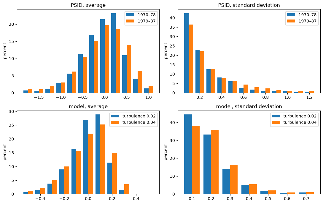
Fig. 26.2 Earnings histograms in the PSID and the model#
Figure 14 of Ljungqvist and Sargent [1998] plots the same histograms for their own panels.
We read the heights of its bars approximately and compare them with ours.
ls_fig14 = {"average": {0.02: [0.5, 1.7, 3.9, 9.0, 16.2, 27.0, 29.7, 10.8, 1.2, 0, 0],
                        0.04: [0.8, 2.3, 5.3, 10.9, 15.0, 22.2, 25.3, 15.0, 3.4, 0, 0]},
            "standard deviation": {0.02: [44.8, 33.2, 14.5, 4.8, 1.9, 0.4, 0.3],
                                   0.04: [38.4, 35.3, 17.5, 5.3, 2.1, 0.7, 0.3]}}
for v, y in ((0.02, y02), (0.04, y04)):
    gaps = [np.abs(percent_histogram(y.mean(axis=1), model_mean_bins)
                   - ls_fig14["average"][v]).max(),
            np.abs(percent_histogram(y.std(axis=1, ddof=1), model_sd_bins)
                   - ls_fig14["standard deviation"][v]).max()]
    print(f"turbulence {v}: largest gaps from their Figure 14, in percentage points, "
          f"{gaps[0]:.1f} (averages) and {gaps[1]:.1f} (standard deviations)")
turbulence 0.02: largest gaps from their Figure 14, in percentage points, 0.8 (averages) and 0.5 (standard deviations)
turbulence 0.04: largest gaps from their Figure 14, in percentage points, 0.9 (averages) and 1.1 (standard deviations)
Our histograms reproduce theirs to within about one percentage point in every bin.
Raising the turbulence parameter from \(0.02\) to \(0.04\) spreads both distributions in the direction that Gottschalk and Moffitt found.
Ljungqvist and Sargent pointed out that the model’s distribution of averages spans a smaller range than the data’s, because their workers are ex ante identical, and that the increase in the model’s standard deviations occurs at lower standard deviations than in the data.
26.4.2. Binding function#
Gottschalk and Moffitt’s decomposition of the model’s earnings at turbulence parameter \(v\) is a pair of numbers \(b(v) = (\sigma^2_\mu(v), \sigma^2_\nu(v))\), the parameters of the m-projection of the model’s distribution of earnings onto the random-effects model.
Gourieroux et al. [1993] call the map \(v \mapsto b(v)\) the binding function; Which Moments to Match? writes it \(\theta^0(\rho)\).
Ljungqvist and Sargent computed the distributions of \(\bar y_i\) and of the men’s standard deviations at \(0.02\) and \(0.04\), whose second moments determine \(b(0.02)\) and \(b(0.04)\), and compared them with the distributions in the data for 1970–78 and 1979–87.
Indirect inference, as Which Moments to Match? describes it, chooses parameter values that make the model’s projection agree with the data’s projection.
We compare the change \(b(v) - b(0.02)\) with the change that Gottschalk and Moffitt measured, because Ljungqvist and Sargent assign the turbulence parameter \(0.02\) to 1970–78 and because the levels of the two projections differ for the reasons given above.
We estimate the binding function by simulating a panel of 10,000 workers at each point of a grid of turbulence parameters, using the same random numbers at every point.
v_grid = np.array([0.0, 0.01, 0.02, 0.03, 0.04, 0.06, 0.1, 0.2, 1.0])
binding = np.array([gm_decomposition(artificial_panel(v)[0]) for v in v_grid])
b02 = binding[v_grid == 0.02][0]
b_uniform = gm_decomposition(artificial_panel(np.inf)[0])   # uniform skill losses

print("turbulence   σ²_μ     σ²_ν    share of the measured change in σ²_μ, σ²_ν")
for v, b in zip(list(v_grid) + [np.inf], list(binding) + [b_uniform]):
    share = (b - b02) / gm_change
    print(f"{v:9.2f} {b[0]:8.4f} {b[1]:8.4f}        {share[0]:6.0%}  {share[1]:6.0%}")
turbulence   σ²_μ     σ²_ν    share of the measured change in σ²_μ, σ²_ν
     0.00   0.0056   0.0493          -12%      1%
     0.01   0.0106   0.0467           -6%     -5%
     0.02   0.0154   0.0489            0%      0%
     0.03   0.0191   0.0512            4%      5%
     0.04   0.0221   0.0547            8%     13%
     0.06   0.0257   0.0577           12%     20%
     0.10   0.0287   0.0612           16%     28%
     0.20   0.0311   0.0643           19%     35%
     1.00   0.0326   0.0678           21%     43%
      inf   0.0329   0.0684           21%     44%
fig, axes = plt.subplots(1, 2, figsize=(11, 4))
for k, (ax, name) in enumerate(zip(axes, ("permanent variance", "transitory variance"))):
    ax.semilogx(v_grid[1:], binding[1:, k] - b02[k], "o-", label="model")
    ax.axhline(gm_change[k], color="k", ls="--", label="PSID, 1979–87 minus 1970–78")
    ax.axhline(0, color="0.7", lw=0.8)
    ax.set_xlabel("turbulence parameter")
    ax.set_title(f"change in {name}")
    ax.legend()
plt.tight_layout()
plt.show()
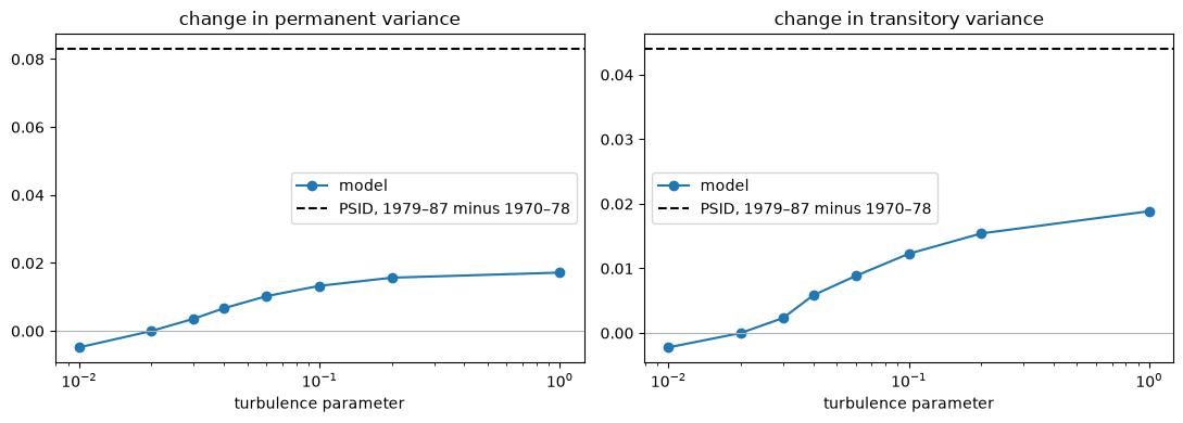
Fig. 26.3 Binding function against the measured changes#
At the turbulence parameter \(0.04\) that Ljungqvist and Sargent assign to 1979–87, the model delivers about 8 percent of the measured increase in the permanent variance and 13 percent of the increase in the transitory variance.
Across random seeds the second share ranges from about 9 to 13 percent, with a mean of about 11 percent.
The binding function rises with turbulence above \(0.01\), and it flattens as the turbulence parameter grows, because the distribution of skill losses approaches the uniform distribution over the skill levels from the lowest to the worker’s current level.
At the largest value in our grid, the model delivers about 21 percent of the increase in the permanent variance and 43 percent of the increase in the transitory variance.
In the limit of uniformly distributed skill losses, the shares are about 21 and 44 percent; across random seeds the second share ranges from about 44 to 49 percent.
Gottschalk and Moffitt trimmed their data, and we have not trimmed the model’s panels.
Trimming each year’s log earnings in the model’s panels in the same way leaves the shares at \(0.04\) roughly unchanged and lowers both shares at the largest turbulence parameter.
y_max, _ = artificial_panel(1.0)
b_trim = {v: gm_decomposition(*trim(y)) for v, y in ((0.02, y02), (0.04, y04),
                                                      (1.0, y_max))}
print(f"turbulence 0.02: σ²_ν {b02[1]:.4f} without trimming, "
      f"{b_trim[0.02][1]:.4f} with trimming")
for v in (0.04, 1.0):
    share = (b_trim[v] - b_trim[0.02]) / gm_change
    print(f"turbulence {v}: shares of the measured changes with trimming "
          f"{share[0]:.0%}, {share[1]:.0%}")
turbulence 0.02: σ²_ν 0.0489 without trimming, 0.0332 with trimming
turbulence 0.04: shares of the measured changes with trimming 8%, 11%
turbulence 1.0: shares of the measured changes with trimming 19%, 35%
The 1 percent tails of each year’s earnings carry about a third of the model’s transitory variance, and trimming lowers the transitory share at the largest turbulence parameter to between 34 and 37 percent across random seeds.
The shares also depend on the range of skills, which bounds a skill loss, and on the speed of skill transitions, which governs how long a loss persists.
Exercise 26.3 shows that with skills on \([1, 3]\) and the original transition probabilities, turbulence delivers about 46 percent of the measured increase in the permanent variance and nearly all of the increase in the transitory variance.
Doubling the transition probabilities as well brings the permanent share back to about one fifth, because laid-off workers regain their skills twice as fast.
Holding the 1970–78 parameter at \(0.02\) also matters.
If the turbulence parameters for both windows are free, the largest changes that the model can deliver are the differences between the largest and smallest points of the binding function.
points = np.vstack([binding, b_uniform])
largest = (points.max(axis=0) - points.min(axis=0)) / gm_change
print(f"largest shares with both windows free: {largest[0]:.0%}, {largest[1]:.0%}")
largest shares with both windows free: 33%, 49%
No value of the turbulence parameter makes the change in the model’s projection equal the change in the data’s projection.
Indirect inference based on these two statistics pushes the turbulence parameter toward the limit in which skill losses are uniformly distributed, and it still leaves a gap.
Ljungqvist and Sargent observed that the increase in their model’s variability occurs at lower standard deviations than in the data; the binding function measures a related shortfall in the sizes of the two variance increases.
They concluded from their comparisons with Gottschalk and Moffitt and with Jacobson, LaLonde, and Sullivan:
The simulations suggest that the mechanism generating high long-term unemployment in our model operates at much lower levels of economic turbulence than those observed in the United States.
Our estimates of the binding function support their inference that the data call for more turbulence than \(0.04\).
They also show that no amount of turbulence in this model reaches the changes in the data, so those changes must also come from components that the model omits.
With the 1970–78 parameter fixed at \(0.02\), the two statistics and the one free parameter leave one overidentifying restriction.
Which Moments to Match? tests a structural model in this way, by asking whether the distance that remains between the projections at the best parameter value exceeds what sampling variation allows.
Here the test is of a joint hypothesis: that the model describes the changes in earnings and that the components of earnings that it omits did not change.
Gottschalk and Moffitt’s suggestion that a rising price of skill may explain the widening dispersion of permanent wages casts doubt on the second part for the permanent variance.
26.5. Layoff rates and turbulence#
The binding function maps a scalar parameter into two numbers, and other structural changes can move those two numbers in the same direction.
We compute the projection of the model with the turbulence parameter held at \(0.02\) and a higher layoff rate \(\lambda\).
b04 = binding[v_grid == 0.04][0]
b_layoff = {λ: gm_decomposition(artificial_panel(0.02, λ=λ)[0])
            for λ in (0.012, 0.015, 0.018, 0.021)}
print("layoff rate   change in σ²_μ, σ²_ν from the 1970–78 calibration")
for λ, b in b_layoff.items():
    print(f"{λ:11.3f}    {b[0] - b02[0]:+.4f}  {b[1] - b02[1]:+.4f}")
print(f"turbulence 0.04:  {b04[0] - b02[0]:+.4f}  {b04[1] - b02[1]:+.4f}")
layoff rate   change in σ²_μ, σ²_ν from the 1970–78 calibration
      0.012    +0.0022  +0.0012
      0.015    +0.0040  +0.0020
      0.018    +0.0060  +0.0026
      0.021    +0.0071  +0.0032
turbulence 0.04:  +0.0067  +0.0058
Doubling or slightly more than doubling the layoff rate raises the permanent variance by about as much as raising the turbulence parameter from \(0.02\) to \(0.04\), and it raises the transitory variance by about \(0.003\) instead of \(0.006\) in this simulation, and by about \(0.002\) instead of \(0.005\) on average across random seeds.
The two explanations project onto nearby points of the random-effects model.
The two explanations’ nearby projections are the identification counterpart of the result in Specification Tests that a comparison of projections has no power against an alternative that leaves the projections equal.
Whether a sample can separate the two explanations depends on the sampling variability of formulas (26.1) in the data.
Gottschalk and Moffitt’s sample contains 2,730 men.
The transitory variance \(\sigma^2_\nu\) is the average of the men’s squared standard deviations \(\hat s_i^2\), so its standard deviation in a sample of 2,730 men is about the standard deviation of \(\hat s_i^2\) divided by \(\sqrt{2730}\).
We compute it from our readings of Gottschalk and Moffitt’s Figure 4, and we compute the power of a test that compares the change in the transitory variance with the change that each explanation predicts.
sd_ν = {}
for window, heights in gm_fig4.items():
    p = np.array(heights) / np.sum(heights)
    s2 = gm_fig4_bins**2
    sd_ν[window] = np.sqrt((p @ s2**2 - (p @ s2)**2) / 2730)
    print(f"{window}: σ²_ν implied by the figure {p @ s2:.3f}, "
          f"standard deviation {sd_ν[window]:.4f}")
sd_change = np.hypot(*sd_ν.values())
gap = (b04[1] - b02[1]) - (b_layoff[0.018][1] - b02[1])
power = ncx2.sf(chi2.ppf(0.95, 1), 1, (gap / sd_change)**2)
print(f"standard deviation of the change {sd_change:.4f}, gap {gap:.4f}, "
      f"power of a 5 percent test {power:.2f}")
1970-78: σ²_ν implied by the figure 0.103, standard deviation 0.0036
1979-87: σ²_ν implied by the figure 0.145, standard deviation 0.0048
standard deviation of the change 0.0060, gap 0.0032, power of a 5 percent test 0.08
Our readings of the figure imply transitory variances of \(0.103\) and \(0.145\), close to the \(0.104\) and \(0.148\) in Gottschalk and Moffitt’s Table 1.
The standard deviation of the change between windows is about \(0.006\), so the difference of about \(0.003\) between the two explanations’ changes in the transitory variance is about half a standard deviation.
This calculation treats the two windows as independent samples of 2,730 men; Gottschalk and Moffitt’s windows contain some of the same men, which lowers the standard deviation of the change, and each window contains fewer than 2,730 men, which raises it.
With the noncentrality calculation of Exercise 25.2, a separation of half a standard deviation gives a 5 percent test a power of about \(0.08\).
The calculation asks whether data generated by one explanation could reject the other.
Both explanations fall more than six standard deviations short of the measured change of \(0.044\), so the calculation measures what the two statistics can identify within the model, not how well either explanation fits.
Gottschalk and Moffitt’s two statistics therefore barely distinguish more frequent layoffs from larger skill losses.
Ljungqvist and Sargent [2008] also compare their model with the earnings losses of displaced workers that Jacobson et al. [1993] measured. They write:
We acknowledge that the substantial earnings losses experienced by displaced U.S. workers since the 1980s by themselves say nothing about increased turbulence between the 1950–1960s and the post 1980s, since that would require evidence from similar displaced worker studies from the 1950–1960s, which unfortunately do not exist.
They add: “Instead, we have drawn support for our story about increased turbulence indirectly from time series studies like that of Gottschalk and Moffitt (1994), whose findings Katz and Autor (1999) showed to be robust across a variety of studies and data sets.”
Each additional statistic adds sufficient statistics to the auxiliary model and shrinks the set of structural parameters whose projections agree with the data’s.
An additional statistic separates two explanations only if the two explanations project onto different values of it, and only if the econometrician computes the statistic in the same way from the model and from the data.
Exercise 26.1 computes displaced-worker statistics for the two explanations.
26.6. Covariance-structure model#
Moffitt and Gottschalk [2011] describe a limitation of the decomposition (26.1):
However, in addition to requiring the choice of arbitrary calendar time intervals, that method is problematic if the permanent variance does not shift abruptly at interval endpoints but instead trends smoothly upward. In that case, deviations from average earnings during the early and later parts of the interval will be incorrectly attributed to transitory earnings.
In terms of the periodogram, a permanent component that changes within a window has power at the nonzero Fourier frequencies, which the projection counts as transitory.
They fit instead a model of the whole covariance structure of earnings, in which a permanent component follows a random walk and a transitory component follows an ARMA(1,1) process,
with loadings and variances that trend over time.
When \(\rho = \theta = 0\), the transitory component is white noise, and the model is the random walk observed with noise of Muth [1960] that Optimal Misspecified Beliefs and The LQ Permanent Income Model use.
They estimate the model by minimum distance with an identity weighting matrix, which fits the model’s autocovariances to the sample autocovariances by least squares.
The chi-squared statistics that they report exceed the 1 percent critical values for every specification, although they judge that the random walk with an ARMA(1,1) transitory component “fits our data adequately.”
We fit a version with constant parameters to the nine-year covariance matrix of our artificial panels, both by least squares, as Moffitt and Gottschalk do, and by minimizing the Gaussian KL divergence.
Its parameters are the variance \(\sigma^2_0\) of the permanent component in the year before the window, the variance \(\sigma^2_\omega\) of its increments, and \(\rho\), \(\theta\), and the variance \(\sigma^2_\xi\) of the innovations \(\xi_{it}\) to the transitory component.
def mg_cov(θ, T=9):
    σ2_0, σ2_ω, ρ, ϑ, σ2_ξ = θ
    t = np.arange(1, T + 1)
    lag = np.abs(np.subtract.outer(t, t))
    γ0 = σ2_ξ * (1 + 2 * ρ * ϑ + ϑ**2) / (1 - ρ**2)
    γ1 = σ2_ξ * (1 + ρ * ϑ) * (ρ + ϑ) / (1 - ρ**2)
    transitory = np.where(lag == 0, γ0, γ1 * ρ**np.maximum(lag - 1, 0))
    return σ2_0 + σ2_ω * np.minimum.outer(t, t) + transitory


def mg_params(p):
    return np.array([np.exp(p[0]), np.exp(p[1]), np.tanh(p[2]), np.tanh(p[3]),
                     np.exp(p[4])])


def mg_projection(S, distance):
    best = None
    for p0 in ([np.log(0.02), np.log(0.002), 0.5, -0.3, np.log(0.02)],
               [np.log(0.01), np.log(0.0005), 1.0, 0.0, np.log(0.04)]):
        objective = lambda p: distance(S, mg_cov(mg_params(p)))
        res = minimize(objective, p0, method="Nelder-Mead",
                       options={"maxiter": 40_000, "xatol": 1e-10, "fatol": 1e-15})
        res = minimize(objective, res.x, method="BFGS")
        if best is None or res.fun < best.fun:
            best = res
    return mg_params(best.x)


print("turbulence  distance       σ²_0     σ²_ω      ρ       θ      σ²_ξ   "
      "permanent  transitory")
for v in (0.02, 0.04):
    y_v = artificial_panel(v, N=40_000, seed=1)[0]
    S = np.cov(y_v.T)
    for name, distance in (("least sq.", euclidean), ("KL", gaussian_kl)):
        θ = mg_projection(S, distance)
        permanent = θ[0] + 5 * θ[1]                   # middle year of the window
        transitory = mg_cov(θ)[4, 4] - permanent
        print(f"{v:9.2f}  {name:10} {θ[0]:8.4f} {θ[1]:8.5f} {θ[2]:7.3f} {θ[3]:7.3f} "
              f"{θ[4]:8.4f} {permanent:9.4f} {transitory:10.4f}")
    print(f"           random effects (ti_gm):  permanent {gm_decomposition(y_v)[0]:.4f}, "
          f"transitory {gm_decomposition(y_v)[1]:.4f}")
turbulence  distance       σ²_0     σ²_ω      ρ       θ      σ²_ξ   permanent  transitory
     0.02  least sq.    0.0015  0.00005   0.649  -0.269   0.0506    0.0017     0.0632
     0.02  KL           0.0020  0.00007   0.633  -0.252   0.0504    0.0023     0.0626
           random effects (ti_gm):  permanent 0.0151, transitory 0.0499
     0.04  least sq.    0.0002  0.00005   0.707  -0.266   0.0553    0.0005     0.0767
     0.04  KL           0.0009  0.00009   0.695  -0.251   0.0550    0.0014     0.0759
           random effects (ti_gm):  permanent 0.0219, transitory 0.0553
The covariance-structure model assigns almost no variance to the permanent component.
It attributes the model’s earnings instability to a transitory component with an annual autoregressive coefficient between \(0.63\) and \(0.71\) and a moving-average coefficient of about \(-0.26\).
Moffitt and Gottschalk’s PSID estimates in their Table 5 are \(\rho = 0.641\) and \(\theta = -0.367\).
The covariance-structure model attributes the increase from turbulence \(0.02\) to \(0.04\) to the transitory component.
The random-effects projection (26.1) of the same panels attributes about half of the increase to the permanent component.
The two auxiliary models disagree because a skill loss at a layoff is large, persistent, and eventually reversed.
A worker who loses half of the accumulated skills regains them at an average rate of one skill level, or \(0.05\), every ten periods of employment, so the worker’s earnings stay low for several years.
A loss of that kind early in a nine-year window lowers the worker’s average and raises the variance of averages across workers, which the random-effects projection counts as permanent.
In terms of the periodogram, a loss that persists for several years puts much of its power at frequency zero.
The covariances of the model’s earnings decline with the lag, and the covariance-structure model fits that decline with its transitory component, so it counts the same loss as transitory.
Moffitt and Gottschalk noted this problem as well: “if the transitory component is serially correlated, the variance of average earnings will be affected by the variance of the transitory component as well.”
The model’s deviations from the workers’ own averages have small serial correlations, like those that Gottschalk and Moffitt found in the PSID.
for v, y in ((0.02, y02), (0.04, y04)):
    d = y - y.mean(axis=1, keepdims=True)
    r = np.corrcoef(d[:, :-1].ravel(), d[:, 1:].ravel())[0, 1]
    print(f"turbulence {v}: correlation of successive deviations {r:.2f}")
turbulence 0.02: correlation of successive deviations 0.17
turbulence 0.04: correlation of successive deviations 0.22
Correlations of \(0.17\) and \(0.22\) between successive deviations are compatible with a transitory component whose autoregressive coefficient is near \(0.7\), so the small correlations in the PSID do not show that its transitory components are close to serially uncorrelated.
The least squares and KL projections onto the covariance-structure model differ in their details.
That model is not an exponential family: its covariance matrices form a curved set, and the argument that made the two projections coincide for the random-effects model does not apply.
26.7. Concluding remarks#
Ljungqvist and Sargent’s comparison of histograms is an informal version of indirect inference: the second moments of their histograms are the parameters of the m-projections of the data and of the structural model onto the same auxiliary model.
For the laissez-faire economy of Ljungqvist and Sargent [1998], the binding function of Gottschalk and Moffitt’s decomposition rises with turbulence above \(0.01\).
With the 1970–78 parameter held at their value of \(0.02\), the binding function cannot reach the changes that Gottschalk and Moffitt measured, and how close it comes depends on the range of skills and on how quickly laid-off workers regain them.
The same two statistics respond in similar ways to an increase in the layoff rate, so they identify turbulence only weakly.
The answer to the question of how much instability is permanent depends on the auxiliary model: the random-effects decomposition and the covariance-structure model of Moffitt and Gottschalk [2011] split the same model-generated instability differently.
26.8. Exercises#
Exercise 26.1
Jacobson et al. [1993] compare the quarterly earnings of workers with six years of tenure who were displaced in the first quarter of 1982 with the earnings of workers who stayed with their employers through 1986.
Ljungqvist and Sargent [1998] construct the model’s counterpart by following, for 11 years, 100,000 workers who have been in the labor force for 20 years. They call the first 12 weeks of year 7 the first quarter of 1982, and they plot the separators whose skill losses exceed 40 percent.
Simulate 100,000 such workers in the laissez-faire economy with turbulence parameter \(0.04\). Identify the stayers, who are employed in every period and never laid off. Identify the separators, who are employed and never laid off in the first six years and are laid off in the first six periods of year 7.
Compute the average 12-week earnings of each group, and the ratio of separators’ to stayers’ earnings over the last two years. Do this for all separators and for the separators whose skill falls by more than 40 percent at the layoff.
Repeat part 2 for all separators in the economy with turbulence parameter \(0.02\) and layoff rate \(0.019\), the layoff rate at which the change in the permanent variance approximately matches the change from raising turbulence to \(0.04\), and compute the fraction of workers with six years of tenure who are displaced at the start of year 7 in each economy.
Which of these statistics can an econometrician compute from data like Jacobson, LaLonde, and Sullivan’s? Which of them distinguish the two explanations?
Solution
Here is one solution.
def displaced_worker_statistics(turbulence, λ=0.009, N=100_000, seed=3):
    m = create_model(turbulence=turbulence, λ=λ)
    rec = simulate_workers(m, *solve_model(m), N=N, T=11 * 26, T_burn=20 * 26,
                           seed=seed)
    emp, laid, h = rec["emp"], rec["laid"], rec["h"]
    k0 = 6 * 26                                        # first period of year 7
    tenured = emp[:, :k0].all(axis=1) & ~laid[:, :k0].any(axis=1)
    stayers = emp.all(axis=1) & ~laid.any(axis=1)
    separators = tenured & laid[:, k0:k0 + 6].any(axis=1)
    rows = np.where(separators)[0]
    k_lay = k0 + laid[rows, k0:k0 + 6].argmax(axis=1)
    loss = np.round(1 - m.h_grid[h[rows, k_lay]] / m.h_grid[h[rows, k_lay - 1]], 9)
    later = np.arange(laid.shape[1])[None, :] > k_lay[:, None]
    big_loss = np.isin(np.arange(N), rows[loss > 0.4])

    def quarterly(mask):
        return rec["earn"][mask][:, :282].reshape(mask.sum(), 47, 6).sum(axis=2).mean(axis=0)

    stay = quarterly(stayers)
    ratio = lambda mask: quarterly(mask)[-8:].mean() / stay[-8:].mean()
    return {"stayers": stayers.sum(), "separators": separators.sum(),
            "shares of separators with losses above 10, 20, 30, 40%":
                np.round([(loss > c).mean() for c in (0.1, 0.2, 0.3, 0.4)], 3),
            "displacement rate": separators.sum() / tenured.sum(),
            "ratio, all separators": ratio(separators),
            "separators with losses above 40%": (loss > 0.4).sum(),
            "later layoffs per separator": (laid[rows] & later).sum(axis=1).mean(),
            "ratio, losses above 40%": ratio(big_loss) if big_loss.any() else np.nan,
            "paths": (stay, quarterly(separators),
                      quarterly(big_loss) if big_loss.any() else None)}


turbulent = displaced_worker_statistics(0.04)
more_layoffs = displaced_worker_statistics(0.02, λ=0.019)
for name, res in (("turbulence 0.04", turbulent),
                  ("turbulence 0.02, layoff rate 0.019", more_layoffs)):
    print(name)
    for key, value in res.items():
        if key != "paths":
            print(f"   {key}: {value:.3f}" if isinstance(value, float)
                  else f"   {key}: {value}")
turbulence 0.04
   stayers: 6048
   separators: 1057
   shares of separators with losses above 10, 20, 30, 40%: [0.549 0.269 0.097 0.025]
   displacement rate: 0.053
   ratio, all separators: 0.825
   separators with losses above 40%: 26
   later layoffs per separator: 0.988
   ratio, losses above 40%: 0.631
turbulence 0.02, layoff rate 0.019
   stayers: 310
   separators: 446
   shares of separators with losses above 10, 20, 30, 40%: [0.397 0.132 0.025 0.002]
   displacement rate: 0.111
   ratio, all separators: 0.787
   separators with losses above 40%: 1
   later layoffs per separator: 2.204
   ratio, losses above 40%: 0.837
fig, ax = plt.subplots()
stay, sep, big = turbulent["paths"]
quarters = np.arange(len(stay)) * 12 / 52 - 6
ax.plot(quarters, stay, label="stayers")
ax.plot(quarters, sep, label="all separators")
ax.plot(quarters, big, label="separators with skill losses above 40%")
ax.set_xlabel("years from the start of year 7")
ax.set_ylabel("12-week earnings")
ax.legend(loc="lower left", fontsize=9)
plt.show()
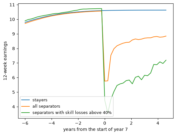
Fig. 26.4 Earnings of stayers and separators#
Ljungqvist and Sargent report 2,889 stayers and 629 separators among their 100,000 workers.
Our simulation has about twice as many stayers and about two thirds more separators.
The shares of separators whose skill losses exceed 10, 20, 30, and 40 percent are 55, 27, 10, and 2.5 percent, against the 47, 25, 11, and 3 percent that they report.
We have not found the source of the difference in the counts.
With turbulence parameter \(0.04\), all separators earn about 17 percent less than stayers three to five years after displacement, and the few separators whose skills fall by more than 40 percent earn about 37 percent less.
Ljungqvist and Sargent describe Jacobson, LaLonde, and Sullivan’s finding as a recovery “toward an eventual level of about 25 percent less than the amount earned at the predisplacement job.”
Their data identify displaced workers by the event of displacement, not by the size of a skill loss, so the earnings statistic that the data can supply is the one for all separators.
Their records cover stayers as well as separators, so data like theirs can also supply a displacement rate.
With the higher layoff rate, all separators earn about 21 percent less than stayers, because after displacement they are laid off again about twice as often as separators in the turbulent economy.
The earnings-loss statistic therefore barely distinguishes the two explanations.
The displacement rate in the economy with the higher layoff rate is about twice the rate in the turbulent economy.
Measured in one period, the rate distinguishes the explanations only if we trust the model’s level of displacement, and throughout this lecture we have compared changes rather than levels.
The change in the displacement rate between two periods distinguishes them: it doubles when the layoff rate doubles and does not move with turbulence.
Measuring that change requires comparable displaced-worker studies from both periods, which is what the passage from Ljungqvist and Sargent [2008] quoted above says is missing.
Exercise 26.2
Let \(y_i\) be a random vector in \(\mathbb{R}^T\) with mean zero and a positive definite covariance matrix \(S\) whose average off-diagonal element is nonnegative, and consider the random-effects family \(N(0, \sigma^2_\mu \mathbf{1}\mathbf{1}^\top + \sigma^2_\nu I)\).
Show that the inverse of \(\Sigma = \sigma^2_\mu \mathbf{1}\mathbf{1}^\top + \sigma^2_\nu I\) is \(\sigma_\nu^{-2} \left(I - c\,\mathbf{1}\mathbf{1}^\top\right)\) with \(c = \sigma^2_\mu / (\sigma^2_\nu + T \sigma^2_\mu)\), and that \(\log p(y_i)\) is a linear function of \(W_i\) and \(T \bar y_i^2\) plus a function of the parameters.
Minimize the Gaussian KL divergence of \(N(0, S)\) from \(N(0, \Sigma)\) over \((\sigma^2_\mu, \sigma^2_\nu)\) and show that the minimizer sets \(\sigma^2_\nu = (\operatorname{tr} S - \mathbf{1}^\top S \mathbf{1}/T)/(T - 1)\) and \(\sigma^2_\mu = \mathbf{1}^\top S \mathbf{1}/T^2 - \sigma^2_\nu / T\).
Show that the least squares projection of \(S\) onto the same family gives the same answer.
Solution
Here is one solution.
For part 1, multiply \(\Sigma\) by \(\sigma_\nu^{-2}(I - c\,\mathbf{1}\mathbf{1}^\top)\) and use \(\mathbf{1}^\top \mathbf{1} = T\): the product is \(I + \sigma_\nu^{-2}\left[\sigma^2_\mu - c(\sigma^2_\nu + T\sigma^2_\mu)\right]\mathbf{1}\mathbf{1}^\top = I\).
Then \(y_i^\top \Sigma^{-1} y_i = \sigma_\nu^{-2}\left(y_i^\top y_i - c T^2 \bar y_i^2\right)\), and \(y_i^\top y_i = W_i + T \bar y_i^2\), so
because \(1 - cT = \sigma^2_\nu / (\sigma^2_\nu + T\sigma^2_\mu)\).
For part 2, the KL divergence of \(N(0, S)\) from \(N(0, \Sigma)\) is minus the expectation of \(\log p(y_i)\) under \(N(0, S)\) plus a constant.
The eigenvalues of \(\Sigma\) are \(\sigma^2_\nu + T\sigma^2_\mu\), with eigenvector \(\mathbf{1}\), and \(\sigma^2_\nu\), with multiplicity \(T - 1\), so \(\log\det\Sigma = \log(\sigma^2_\nu + T\sigma^2_\mu) + (T - 1)\log\sigma^2_\nu\).
With \(E[W_i] = \operatorname{tr} S - \mathbf{1}^\top S \mathbf{1}/T\) and \(E[T\bar y_i^2] = \mathbf{1}^\top S \mathbf{1}/T\), the objective separates into a function of \(a = \sigma^2_\nu\) and a function of \(d = \sigma^2_\nu + T\sigma^2_\mu\):
Minimizing gives \(a = E[W_i]/(T-1)\) and \(d = E[T\bar y_i^2]\), which are the stated formulas.
For part 3, the least squares problem \(\min \sum_{t \le s} (S_{ts} - \Sigma_{ts})^2\) separates into the diagonal elements, all equal to \(\sigma^2_\mu + \sigma^2_\nu\), and the off-diagonal elements, all equal to \(\sigma^2_\mu\).
The minimizer sets \(\sigma^2_\mu + \sigma^2_\nu\) equal to the average diagonal element \(\bar s_d\) and \(\sigma^2_\mu\) equal to the average off-diagonal element \(\bar s_o\).
Since \(\operatorname{tr} S = T \bar s_d\) and \(\mathbf{1}^\top S \mathbf{1} = T\bar s_d + T(T - 1)\bar s_o\), the formulas of part 2 give \(\sigma^2_\nu = \bar s_d - \bar s_o\) and \(\sigma^2_\mu = \bar s_o\).
So \(\sigma^2_\mu \geq 0\) exactly when the average off-diagonal element of \(S\) is nonnegative, which is why the exercise assumes it.
S = np.cov(y04.T)
T = len(S)
s_d, s_o = np.mean(np.diag(S)), (S.sum() - np.trace(S)) / (T * (T - 1))
print("least squares:", np.round([s_o, s_d - s_o], 6))
σ2_ν = (np.trace(S) - S.sum() / T) / (T - 1)
print("KL formulas:  ", np.round([S.sum() / T**2 - σ2_ν / T, σ2_ν], 6))
least squares: [0.022123 0.054737]
KL formulas:   [0.022123 0.054737]
Exercise 26.3
Ljungqvist and Sargent [1998] report that “similar results were obtained in earlier simulations in which we had doubled both the range of skills and the transition probabilities of gaining a skill level when remaining employed for two periods and of losing a skill level when being unemployed for two consecutive periods.”
Set the skills on \([1, 3]\), keep 21 skill levels and the original transition probabilities, and recompute the binding function at the turbulence parameters \(0.02\), \(0.04\), \(0.1\), and \(1\).
Also double the probability of a skill gain to \(0.2\) and the probability of a skill loss to \(0.4\), and recompute the binding function.
Part 2 is our reading of their sentence; part 1 separates the effect of the range from the effect of the transition probabilities.
What fractions of the measured changes in the permanent and transitory variances can turbulence deliver in each case, and why do the two cases differ?
Solution
Here is one solution.
grid, ends = (0.02, 0.04, 0.1, 1.0), (0.02, 1.0)
cases = (("wider range", dict(h_max=3.0), grid),
         ("wider range, faster transitions", dict(h_max=3.0, up=0.2, down=0.4), grid),
         ("wider range, faster skill gains only", dict(h_max=3.0, up=0.2), ends),
         ("wider range, faster skill losses only", dict(h_max=3.0, down=0.4), ends))
for case, kwargs, v_wide in cases:
    b_wide = np.array([gm_decomposition(artificial_panel(v, **kwargs)[0])
                       for v in v_wide])
    print(case)
    for v, b in zip(v_wide, b_wide):
        share = (b - b_wide[0]) / gm_change
        print(f"   turbulence {v:5.2f}: σ²_μ {b[0]:.4f}, σ²_ν {b[1]:.4f}, "
              f"shares of the measured changes {share[0]:.0%}, {share[1]:.0%}")
wider range
   turbulence  0.02: σ²_μ 0.0230, σ²_ν 0.0556, shares of the measured changes 0%, 0%
   turbulence  0.04: σ²_μ 0.0372, σ²_ν 0.0689, shares of the measured changes 17%, 30%
   turbulence  0.10: σ²_μ 0.0514, σ²_ν 0.0853, shares of the measured changes 34%, 68%
   turbulence  1.00: σ²_μ 0.0608, σ²_ν 0.0987, shares of the measured changes 46%, 98%
wider range, faster transitions
   turbulence  0.02: σ²_μ 0.0136, σ²_ν 0.0558, shares of the measured changes 0%, 0%
   turbulence  0.04: σ²_μ 0.0195, σ²_ν 0.0683, shares of the measured changes 7%, 28%
   turbulence  0.10: σ²_μ 0.0263, σ²_ν 0.0872, shares of the measured changes 15%, 71%
   turbulence  1.00: σ²_μ 0.0311, σ²_ν 0.1033, shares of the measured changes 21%, 108%
wider range, faster skill gains only
   turbulence  0.02: σ²_μ 0.0110, σ²_ν 0.0631, shares of the measured changes 0%, 0%
   turbulence  1.00: σ²_μ 0.0284, σ²_ν 0.1021, shares of the measured changes 21%, 89%
wider range, faster skill losses only
   turbulence  0.02: σ²_μ 0.0307, σ²_ν 0.0506, shares of the measured changes 0%, 0%
   turbulence  1.00: σ²_μ 0.0649, σ²_ν 0.1011, shares of the measured changes 41%, 115%
A wider range of skills allows larger skill losses.
With skills on \([1, 3]\) and the original transition probabilities, turbulence delivers up to about 46 percent of the measured increase in the permanent variance and nearly all of the increase in the transitory variance.
Doubling the transition probabilities as well halves the time that a laid-off worker needs to regain the lost skill levels.
A skill loss then lasts a smaller part of a nine-year window and lowers the worker’s average by less, so the random-effects projection counts less of it as permanent.
In that case turbulence delivers at most about one fifth of the increase in the permanent variance, as in the original economy, and slightly more than all of the increase in the transitory variance.
The faster recovery is what matters: doubling only the probability of a skill gain lowers the permanent share at turbulence \(1\) to about 21 percent, while doubling only the probability of a skill loss leaves it at about 41 percent.
Ljungqvist and Sargent’s sentence concerns their qualitative findings; the binding function shows that the permanent share is not robust to changing the range of skills alone.