24. Approximation Errors in Time Series Models#
24.1. Overview#
When an econometrician estimates a model that does not contain the process that generated the data, the maximum likelihood estimator converges, under regularity conditions, to the member of the model that is closest to the true process in the sense of Kullback–Leibler (KL) divergence.
In Information Projections we called that member the m-projection of the true distribution onto the model.
We organize this lecture around one consequence of that fact: by choosing the model, the data, and any filter that transforms the data, an econometrician chooses which projection an estimator computes.
For stationary Gaussian processes, the KL divergence per observation converges to an integral over frequencies, so the m-projection trades off approximation errors at different frequencies.
Sims [1971], Sims [1974], Sims [1993], and Hansen and Sargent [1993] study the errors that an econometrician makes when fitting a misspecified time series model, and they show how sampling, seasonal noise, and seasonal adjustment change those errors.
The lecture has five sections.
Kullback–Leibler divergence between Gaussian processes describes the KL divergence between two stationary Gaussian processes as an integral over frequencies.
Misspecified autoregressions describes misspecified autoregressions as projections of spectral densities, and describes how filtering the data and the model, filtering the data alone, and deleting frequency bands change the projection.
Distributed lags describes least squares estimates of distributed lags as m-projections weighted by the spectral density of the regressor, and describes Sims’s results on sampling and on seasonal noise.
Seasonal adjustment in dynamic models describes seasonal adjustment in dynamic rational expectations models.
Garbling and the data processing inequality treats filtering, deleting frequency bands, removing seasonal means, and sampling as garblings in the sense of Blackwell’s Theorem on Comparing Experiments, and uses the data processing inequality to organize the results of the earlier sections.
Specification Tests continues this lecture: it describes specification tests as comparisons of two projections.
Each section uses the notation of the papers that it describes, so a few symbols change meaning from one section to another.
In particular, \(A\) denotes Hansen and Sargent’s criterion and Sims’s moving-average operator; \(c\) denotes a filter, Sims’s lag distribution of seasonal noise, and consumption; \(w\) denotes a finite Fourier transform and Sims’s seasonal noise; \(Y\) denotes a sampled series and income; \(\gamma\) denotes an autocovariance and a productivity parameter; \(d\) denotes a lag distribution and an endowment shock; and \(v\) denotes the seasonal innovation and Sims’s noise in \(z\).
The lecture on covariance stationary processes describes spectral densities.
Optimal Misspecified Beliefs uses Hansen and Sargent’s criterion (24.4) to compute the beliefs of agents who forecast with a misspecified model.
We use the following imports.
import numpy as np
import matplotlib.pyplot as plt
from scipy import integrate
from scipy.linalg import toeplitz, cho_factor, cho_solve
from scipy.optimize import minimize
24.2. Kullback–Leibler divergence between Gaussian processes#
24.2.1. Spectral densities#
Let \(\{y_t\}\) be a covariance stationary process with mean zero and autocovariances \(\gamma_k = E[y_t y_{t-k}]\).
Its spectral density is
We follow the convention of Hansen and Sargent [1993].
Two Illustrations of the Quantity Theory of Money and Drifts and Volatilities put a factor \(1/(2\pi)\) in front of the sum; the factor rescales \(f\) and leaves ratios such as \(f/g\) unchanged.
Setting \(k = 0\) in the second formula shows that \(f\) distributes the variance \(\gamma_0\) of \(y_t\) across frequencies \(\omega \in [-\pi, \pi]\).
The first-order autoregression \(y_t = \rho y_{t-1} + \sigma \varepsilon_t\) with \(|\rho| < 1\) and white noise \(\varepsilon_t\) of unit variance has spectral density \(\sigma^2 / |1 - \rho e^{-i\omega}|^2\).
More generally, the autoregression \(a(L) y_t = \sigma \varepsilon_t\) with \(a(L) = 1 - a_1 L - \cdots - a_p L^p\) has spectral density \(\sigma^2 / |a(e^{-i\omega})|^2\).
We evaluate spectral densities on a fine grid of frequencies in \([0, 2\pi)\), on which the average of a function approximates \(\frac{1}{2\pi}\) times its integral over a period.
n_grid = 2**14
ω = 2 * np.pi * (np.arange(n_grid) + 0.5) / n_grid
z = np.exp(-1j * ω)


def ar_poly(a):
    """a(e^{-iω}) = 1 - a_1 e^{-iω} - ... - a_p e^{-ipω} on the grid."""
    return 1 - sum(a_j * z**(j + 1) for j, a_j in enumerate(np.atleast_1d(a)))


def ar_spectrum(a, σ2=1.0):
    return σ2 / np.abs(ar_poly(a))**2


def autocov(f, n_lags):
    """γ_0, ..., γ_{n_lags} from the spectral density f on the grid."""
    return np.array([np.mean(f * np.cos(ω * k)) for k in range(n_lags + 1)])


def kl_rate(f, g, keep=None):
    """(1/4π) ∫ [f/g - 1 - log(f/g)] dω over the frequencies in keep."""
    ratio = f / g
    integrand = ratio - 1 - np.log(ratio)
    if keep is not None:
        integrand = np.where(keep, integrand, 0.0)
    return 0.5 * np.mean(integrand)
24.2.2. Divergence rate#
Let \(f\) and \(g\) be the spectral densities of two stationary Gaussian processes with mean zero, and suppose that both are bounded and bounded away from zero.
Under the first process, the vector \(y^T = (y_1, \ldots, y_T)\) of the first \(T\) observations is \(N(0, \Gamma_T(f))\), where \(\Gamma_T(f)\) is the \(T \times T\) matrix with entries \(\gamma_{j-k}\); under the second it is \(N(0, \Gamma_T(g))\).
The KL divergence between these two multivariate normal distributions is \(\frac{1}{2}[\operatorname{tr}(\Gamma_T(g)^{-1}\Gamma_T(f)) - T - \log\det(\Gamma_T(g)^{-1}\Gamma_T(f))]\), and it grows approximately in proportion to \(T\).
Divided by \(T\), it converges to
We call \(D(f \| g)\) the KL divergence rate of the process with spectral density \(f\) from the process with spectral density \(g\).
Likelihood Ratio Processes and Likelihood Processes For VAR Models write this rate \(h_{KL}(f, g)\) and compute it in the time domain, for Markov chains and for Gaussian vector autoregressions; for two first-order vector autoregressions with mean zero, the vector formula (24.3) below equals (29.4).
The KL divergence rate is the average over frequencies of the KL divergences between normal distributions whose variances are the two spectral densities at each frequency.
The transforms \(w_j = T^{-1/2} \sum_{t=1}^T y_t e^{-i \omega_j t}\) at the frequencies \(\omega_j = 2\pi j / T\) with \(0 < \omega_j < \pi\) are, for large \(T\), approximately independent complex normal random variables with variances \(f(\omega_j)\).
So the KL divergence between the two distributions of a sample of \(T\) observations is approximately the sum, over about \(T/2\) frequencies, of the divergences between the two distributions of \(w_j\).
At each frequency, the divergence is the divergence between two normal distributions with mean zero and variances \(f(\omega_j)\) and \(g(\omega_j)\), which by formula (22.16) of Exponential Family and Maximum Entropy is \(\frac{1}{2}[f/g - 1 - \log(f/g)]\) for a real normal random variable and twice that for a complex one.
Summing over the \(T/2\) frequencies and dividing by \(T\) gives (24.2).
We check (24.2) by computing the exact divergence between the distributions of \(T\) observations from two first-order autoregressions with \(\rho = 0.9\) and \(\rho = 0.5\).
def ar1_autocov(ρ, T):
    return ρ**np.arange(T) / (1 - ρ**2)


def kl_normal_vectors(Σ1, Σ2):
    """KL divergence of N(0, Σ1) from N(0, Σ2)."""
    M = cho_solve(cho_factor(Σ2), Σ1)
    return 0.5 * (np.trace(M) - len(M) - np.linalg.slogdet(M)[1])


ρ1, ρ2 = 0.9, 0.5
for T in (25, 100, 400, 1600):
    Σ1 = toeplitz(ar1_autocov(ρ1, T))
    Σ2 = toeplitz(ar1_autocov(ρ2, T))
    print(f"T = {T:5d}:  divergence / T = {kl_normal_vectors(Σ1, Σ2) / T:.5f}")
print(f"divergence rate:       {kl_rate(ar_spectrum(ρ1), ar_spectrum(ρ2)):.5f}")
T =    25:  divergence / T = 0.43570
T =   100:  divergence / T = 0.42471
T =   400:  divergence / T = 0.42197
T =  1600:  divergence / T = 0.42128
divergence rate:       0.42105
For a vector process with spectral density matrices \(F\) and \(G\) and means \(\nu\) and \(\mu\), the same argument gives
where \(n\) is the dimension of the process.
The means enter through the transform at frequency zero, \(w_0 = T^{1/2} \bar y\), whose covariance matrix is approximately \(G(0)\) under the second process.
Optimal Misspecified Beliefs describes a model with mean zero that fits a nonzero mean by raising \(G(0)\), which shrinks the mean term.
24.2.3. Hansen and Sargent’s approximation criterion#
Hansen and Sargent [1993] write:
We want to study the errors of economic interpretation that an econometrician makes when he estimates a misspecified model. It is well-known that there is an important link between likelihood estimation and the Kullback–Leibler (1951) information criterion.
They let \(F(\omega)\) and \(\nu\) be the spectral density matrix and mean of a vector of observables, and \(G(\omega, \delta)\) and \(\mu(\delta)\) be the spectral density matrix and mean that an approximating model with parameter vector \(\delta\) implies.
They show that, when the minimizer is unique, the Gaussian maximum likelihood estimator of \(\delta\) converges almost surely to the minimizer of their approximation criterion
Subtracting from \(A(\delta)\) the quantity \(\frac{1}{2\pi}\int \log \det F(\omega) \, d\omega + n\), which does not depend on \(\delta\), leaves twice the divergence rate (24.3).
Hence the probability limit of the misspecified maximum likelihood estimator is the m-projection of the true process onto the model, with divergence measured by the KL divergence rate.
Hansen and Sargent [1993] apply at each frequency \(\omega\) what they call “the familiar information inequality for normally distributed random variable”:
Integrating over frequencies shows that the first two terms of \(A(\delta)\) are at least \(\frac{1}{2\pi}\int \log \det F(\omega) \, d\omega + n\), with equality when \(G(\cdot, \delta) = F\); the mean term is nonnegative and equals zero when \(\mu(\delta) = \nu\).
24.2.4. Periodogram and likelihood#
Hansen and Sargent [1980], following Hannan [1970], use a frequency-domain approximation to the Gaussian log likelihood of a sample of \(T\) observations, often called the Whittle likelihood after Whittle [1953]:
plus a constant, where \(\omega_j = 2\pi j / T\) and \(I(\omega_j) = T^{-1} \left(\sum_t y_t e^{-i\omega_j t}\right)\left(\sum_t y_t e^{i\omega_j t}\right)^\top\) is the periodogram.
Hansen and Sargent write \(S\) for the model’s spectral density matrix; we keep the notation \(G(\omega, \delta)\) of their 1993 paper.
The Kalman Filter and Vector Autoregressions evaluates the exact Gaussian log likelihood of a state-space model from its innovations; (24.5) approximates the same likelihood frequency by frequency.
Maximizing (24.5) minimizes a sample version of the first two terms of (24.4), with the periodogram in place of the true spectral density \(F\).
In Information Projections the maximum likelihood estimator is the m-projection of the empirical distribution onto the model; in (24.5) the periodogram takes the place of the empirical distribution.
The periodogram does not converge to \(F(\omega)\) at any frequency: for a scalar process its variance stays near \(f(\omega)^2\).
Averages of \(\operatorname{tr}[G(\omega_j, \delta)^{-1} I(\omega_j)]\) over frequencies do converge to the corresponding averages of \(\operatorname{tr}[G(\omega, \delta)^{-1}F(\omega)]\), and the convergence of the estimator to the minimizer of (24.4) requires only those averages.
24.3. Misspecified autoregressions#
24.3.1. Projection onto autoregressions#
Suppose that an econometrician fits the autoregression \(a(L) y_t = \sigma \varepsilon_t\) to a scalar process with spectral density \(f\), so that the model’s spectral density is \(g(\omega) = \sigma^2 / |a(e^{-i\omega})|^2\).
For a fixed polynomial \(a\), the variance \(\sigma^2\) that minimizes the divergence rate (24.2) is
the mean squared one-step-ahead forecast error of the rule \(\hat y_t = a_1 y_{t-1} + \cdots + a_p y_{t-p}\).
When the roots of \(a\) lie outside the unit circle, Kolmogorov’s formula gives \(\frac{1}{2\pi}\int \log |a(e^{-i\omega})|^2 \, d\omega = 0\).
Substituting \(\sigma^2(a)\) into (24.2) then gives
By Kolmogorov’s formula, \(\frac{1}{2\pi}\int_{-\pi}^{\pi} \log f(\omega) \, d\omega = \log \sigma^2_\infty\), where \(\sigma^2_\infty\) is the variance of the one-step-ahead forecast error of \(y_t\) given its infinite past, so \(D(f \| g) = \frac{1}{2} \log [\sigma^2(a)/\sigma^2_\infty]\).
For a vector process, the spectral factorization identity (57.24) of The Kalman Filter and Vector Autoregressions gives the counterpart: the average over frequencies of the log determinant of the spectral density matrix of a state-space model’s observables equals the log determinant of its innovation covariance matrix, \(G\Sigma G^\top + R\) in that lecture’s notation.
The second term does not depend on \(a\), so the m-projection of a stationary process onto the autoregressions of order \(p\) chooses the coefficients that minimize the mean squared one-step-ahead forecast error.
Those coefficients solve the Yule–Walker equations \(\sum_{k=1}^p a_k \gamma_{j-k} = \gamma_j\) for \(j = 1, \ldots, p\); for \(p = 1\), \(a_1 = \gamma_1 / \gamma_0\).
In the frequency-domain likelihood (24.5), the autoregressions of order \(p\) form an exponential family whose sufficient statistics are the autocovariances at lags \(0, \ldots, p\).
As in Information Projections, the m-projection matches moments: its autocovariances at lags \(0, \ldots, p\) equal those of \(y_t\).
The same argument applies to any model whose moving-average operator is a ratio of polynomials with leading coefficient one and roots outside the unit circle; with a nonzero mean, the concentrated variance adds the squared mean of the forecast errors.
Optimal Misspecified Beliefs uses it to compute the forecasting rules of agents whose models are misspecified.
The function below computes the m-projection by minimizing the divergence rate directly.
Its argument keep restricts the criterion to a subset of frequencies.
Replacing a root of \(a\) by its reciprocal leaves the shape of the spectral density unchanged, so the criterion also has minimizers outside the stationary region.
We restrict the search to stationary autoregressions by parameterizing them with partial autocorrelations in \((-1, 1)\).
def yule_walker(γ, p):
    return np.linalg.solve(toeplitz(γ[:p]), γ[1:p + 1])


def pacf_to_ar(pacf):
    """AR coefficients from partial autocorrelations (Durbin–Levinson)."""
    a = np.zeros(0)
    for φ_kk in pacf:
        a = np.append(a - φ_kk * a[::-1], φ_kk)
    return a


def ar_to_pacf(a):
    a, pacf = np.array(a, dtype=float), []
    while len(a):
        φ_kk = a[-1]
        pacf.append(φ_kk)
        a = (a[:-1] + φ_kk * a[:-1][::-1]) / (1 - φ_kk**2)
    return np.array(pacf[::-1])


def ar_projection(f, p, keep=None):
    """Stationary AR(p) coefficients and innovation variance that minimize
    the divergence rate of f from the AR model, over the frequencies in keep."""
    keep = np.ones(n_grid, bool) if keep is None else keep

    def criterion(θ):
        a2 = np.abs(ar_poly(pacf_to_ar(np.tanh(θ)))[keep])**2
        return np.log(np.mean(f[keep] * a2)) - np.mean(np.log(a2))

    θ0 = np.arctanh(ar_to_pacf(yule_walker(autocov(f, p), p)))
    θ = minimize(criterion, θ0, method="BFGS", options={"gtol": 1e-8}).x
    a = pacf_to_ar(np.tanh(θ))
    σ2 = np.mean((f * np.abs(ar_poly(a))**2)[keep])
    return a, σ2
24.3.2. Seasonal example#
Let the observed quarterly series be the sum \(y_t = x_t + s_t\) of a nonseasonal component and a seasonal component that are independent of each other:
The roots of the seasonal polynomial lie just outside the unit circle at the seasonal frequencies \(\pi/2\) and \(\pi\), so the spectral density of \(s_t\) has narrow peaks there.
We scale \(v_t\) so that the variance of \(s_t\) is one quarter of the variance of \(x_t\).
An econometrician fits a first-order autoregression to \(y_t\).
ρ_x, φ = 0.9, 0.98
f_x = ar_spectrum(ρ_x)
f_s = ar_spectrum([-φ, -φ**2, -φ**3])
f_s = f_s * 0.25 * np.mean(f_x) / np.mean(f_s)
f_y = f_x + f_s

a_full, σ2_full = ar_projection(f_y, 1)
g_full = ar_spectrum(a_full, σ2_full)
γ_y = autocov(f_y, 1)
print(f"m-projection: ρ* = {a_full[0]:.4f},  γ_1/γ_0 = {γ_y[1] / γ_y[0]:.4f}")
print(f"divergence rate at the projection: {kl_rate(f_y, g_full):.4f}")
print(f"g/f at frequency zero: {g_full[0] / f_y[0]:.2f}")
m-projection: ρ* = 0.6200,  γ_1/γ_0 = 0.6200
divergence rate at the projection: 0.4291
g/f at frequency zero: 0.28
The m-projection has \(\rho^* = 0.62\), well below the coefficient \(0.9\) of the nonseasonal component.
The left panel of the figure plots the logarithms of the spectral densities of \(y_t\), of \(x_t\), and of the projection.
The right panel plots \(\frac{1}{2}[f/g - 1 - \log(f/g)]\) at each frequency; its average over frequencies is the divergence rate.
In the right panel, vertical lines mark the seasonal frequencies \(\pi/2\) and \(\pi\).
half = ω <= np.pi
π_ticks = (np.arange(5) * np.pi / 4,
           ["0", r"$\pi/4$", r"$\pi/2$", r"$3\pi/4$", r"$\pi$"])

fig, axes = plt.subplots(1, 2, figsize=(11, 4))
ax = axes[0]
ax.plot(ω[half], np.log(f_y[half]), lw=2, label="$y_t$")
ax.plot(ω[half], np.log(f_x[half]), "--", label="$x_t$")
ax.plot(ω[half], np.log(g_full[half]), lw=2,
        label=rf"AR(1) projection, $\rho^*$ = {a_full[0]:.2f}")
ax.set_xticks(*π_ticks)
ax.set_xlabel(r"$\omega$")
ax.set_ylabel("log spectral density")
ax.legend(loc="lower center", bbox_to_anchor=(0.5, 1.0), ncol=2, fontsize=9,
          frameon=False)

ax = axes[1]
ratio = f_y / g_full
ax.semilogy(ω[half], 0.5 * (ratio - 1 - np.log(ratio))[half], lw=2)
ax.set_ylim(1e-3, 30)
ax.set_xticks(*π_ticks)
ax.set_xlabel(r"$\omega$")
ax.set_ylabel(r"KL divergence at frequency $\omega$")
for c in (np.pi / 2, np.pi):
    ax.axvline(c, color="0.7", lw=0.8)
plt.tight_layout()
plt.show()
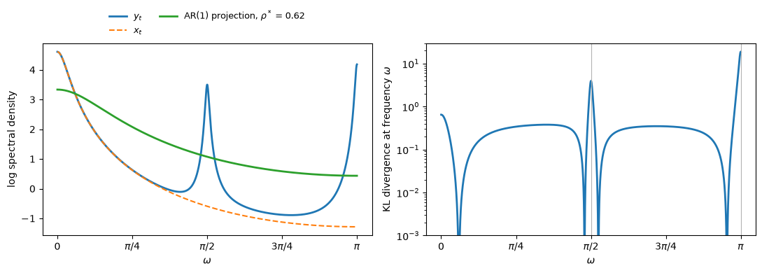
Fig. 24.1 AR(1) projection of a seasonal series#
A first-order autoregression cannot produce a peak at \(\pi/2\), and it can produce a narrow peak at \(\pi\) only with a coefficient near \(-1\), which would give up the power near frequency zero.
So the divergence is largest at those two frequencies.
For a given \(\sigma^2\), lowering \(\rho\) raises the model’s spectral density at high frequencies and lowers it near frequency zero.
The first effect reduces the divergence at \(\pi/2\) and \(\pi\); the second raises it near frequency zero, where \(x_t\) has most of its power.
With \(r = f/g\), the integrand \(\frac{1}{2}(r - 1 - \log r)\) grows linearly in \(r\) and only logarithmically in \(1/r\), so understating the spectral density at the seasonal peaks costs more than overstating it elsewhere; Likelihood Processes For VAR Models makes the same observation about shock variances.
At \(\rho^* = 0.62\) the projection’s spectral density at frequency zero is about 28 percent of the spectral density of \(y_t\).
24.3.3. Deleting seasonal bands#
Hansen and Sargent [1993] describe what they call ideal seasonal adjustment.
Let \(K\) be the set of frequencies outside bands around the seasonal frequencies, and let \(1_K(\omega)\) equal one for \(\omega \in K\) and zero otherwise; Hansen and Sargent write \(C(\omega)\) for this indicator.
They replace (24.4) by
With the seasonal bands deleted, the econometrician projects the part of the process that lies outside the bands onto the part of the model that lies outside them.
The divergence rate restricted to \(K\) is at most the full divergence rate, because the information inequality makes every deleted term nonnegative; Garbling and the data processing inequality reads this inequality as an instance of the data processing inequality.
If, for some \(\delta_0\), the model matches \(F\) outside the seasonal bands and matches the mean, \(\mu(\delta_0) = \nu\), then \(\delta_0\) is among the minimizers of (24.6), whatever the model does inside the bands.
Hansen and Sargent add that omitting frequencies might hinder identification by introducing additional minimizers, and that, when the model remains identified, omitting frequencies will typically increase the asymptotic variance of the estimator unless the seasonal frequencies are contaminated by measurement error.
When the model is correctly specified at all frequencies, the estimator that uses all frequencies is efficient, and by Hausman’s lemma the increase in asymptotic variance equals the variance of the difference between the two estimators.
Specification Tests turns that difference into a test.
In our example, no first-order autoregression matches the spectral density of \(y_t\) outside the bands, because the seasonal component has some power at every frequency.
But about 94 percent of the seasonal component’s variance lies in bands of width \(\pi/8\) around the seasonal frequencies.
def seasonal_keep(Δ):
    """True outside bands of width Δ centered on π/2, π, and 3π/2."""
    def dist(c):
        return np.minimum(np.abs(ω - c), 2 * np.pi - np.abs(ω - c))
    inside = ((dist(np.pi / 2) < Δ / 2) | (dist(np.pi) < Δ / 2)
              | (dist(3 * np.pi / 2) < Δ / 2))
    return ~inside


keep_8 = seasonal_keep(np.pi / 8)
print(f"share of the seasonal variance in bands of width π/8: "
      f"{1 - np.mean(f_s * keep_8) / np.mean(f_s):.2f}")
print(f"divergence rate of the AR(1) projection: all frequencies "
      f"{kl_rate(f_y, g_full):.4f}, outside the bands "
      f"{kl_rate(f_y, g_full, keep_8):.4f}")
for Δ in (np.pi / 16, np.pi / 8, np.pi / 4):
    a_K, _ = ar_projection(f_y, 1, seasonal_keep(Δ))
    print(f"band width {Δ / np.pi:.4f}π:  ρ* = {a_K[0]:.4f}")
share of the seasonal variance in bands of width π/8: 0.94
divergence rate of the AR(1) projection: all frequencies 0.4291, outside the bands 0.2287
band width 0.0625π:  ρ* = 0.8520
band width 0.1250π:  ρ* = 0.8733
band width 0.2500π:  ρ* = 0.8850
Deleting bands of width \(\pi/8\) raises \(\rho^*\) from \(0.62\) to \(0.87\).
The remaining gap between \(0.87\) and \(0.9\) comes from seasonal power that lies outside the deleted bands, and it shrinks as the bands widen.
24.3.4. Filtering#
Let \(c(L)\) be a filter whose frequency response \(c(e^{-i\omega})\) never equals zero.
Filtering the data by \(c(L)\) multiplies \(f\) by \(|c(e^{-i\omega})|^2\), and filtering the model by \(c(L)\) multiplies \(g\) by the same factor.
The ratio \(f/g\) at each frequency is unchanged, so filtering the data and the model by the same invertible filter leaves the divergence rate (24.2) and the projection unchanged.
Two other operations change the projection.
Deleting frequencies, as in (24.6), removes the bands from the criterion and leaves the other frequencies unchanged. In a regression, filtering both variables with a filter that is zero in the bands and one elsewhere is equivalent to deleting the bands. That filter is not invertible, so the invariance argument does not apply.
Filtering the data but not the model replaces \(f\) by \(|c(e^{-i\omega})|^2 f\) and leaves \(g\) alone, so the econometrician projects a different process onto the same model.
Garbling and the data processing inequality shows that the invariance and the effect of deleting frequencies are the equality and inequality cases of the data processing inequality, which says nothing about filtering the data alone.
The code below confirms the invariance and computes the effect of filtering the data alone by \(c(L) = 1 - 0.5L\).
c2 = np.abs(1 - 0.5 * z)**2
print(f"D(f || g) = {kl_rate(f_y, g_full):.6f},  "
      f"D(|c|²f || |c|²g) = {kl_rate(c2 * f_y, c2 * g_full):.6f}")
a_c, _ = ar_projection(c2 * f_y, 1)
print(f"AR(1) projection of the data filtered by 1 - 0.5L: ρ* = {a_c[0]:.4f}")
print(f"share of the filtered variance from the seasonal component: "
      f"{np.mean(c2 * f_s) / np.mean(c2 * f_y):.2f}")
D(f || g) = 0.429093,  D(|c|²f || |c|²g) = 0.429093
AR(1) projection of the data filtered by 1 - 0.5L: ρ* = -0.0777
share of the filtered variance from the seasonal component: 0.56
The filter multiplies \(f\) by \(|1 - 0.5 e^{-i\omega}|^2 = 1.25 - \cos\omega\).
It cuts the spectral density at frequency zero, where \(x_t\) has most of its power, to one quarter, and it multiplies the spectral density at the seasonal peak \(\pi\) by \(2.25\).
The seasonal component, whose first-order autocorrelation is negative, then accounts for more than half of the variance of the filtered series, and the AR(1) projection of the filtered series has \(\rho^* = -0.08\).
24.4. Distributed lags#
24.4.1. Least squares as weighted projection#
Let
where \(\{x_t\}\) and \(\{u_t\}\) are stationary and \(u_t\) is uncorrelated with \(x_{t-s}\) for every \(s\).
Write \(\tilde b(\omega) = \sum_s b_s e^{-i\omega s}\) for the Fourier transform of the lag distribution and \(S_x\) for the spectral density of \(x\).
An econometrician estimates the lag distribution by least squares, subject to constraints such as a finite length or a parametric form.
In large samples the constrained estimate \(\hat b\) converges to the lag distribution \(d\) that minimizes
over the lag distributions that satisfy the constraints.
Least squares is the maximum likelihood estimator for the Gaussian model in which \(y_t\), given the path of \(x\), has mean \(\sum_s d_s x_{t-s}\) and serially uncorrelated deviations with variance \(\sigma^2\).
Minimizing the KL divergence rate of the true conditional distribution from this model over \(\sigma^2\) leaves one half the logarithm of the mean squared error (24.8), plus a term that does not depend on the lag distribution \(d\).
The constrained least squares estimator therefore converges to the m-projection of the true conditional distribution onto the constrained model.
The spectral density \(S_x\) weights the projection: errors in \(\tilde d\) cost most at the frequencies at which \(x\) has most of its power.
24.4.2. Sampling continuous-time lags#
Sims [1971] studies a continuous-time distributed lag \(y(t) = \int b(s) x(t - s) \, ds + u(t)\) observed at integer dates \(t\).
He uses the Fourier transform \(\tilde b(\omega) = \int e^{-i\omega t} b(t) \, dt\) and the spectral density \(S_x\) of the continuous-time process \(x\), both defined on the whole real line.
Sampling at integer dates makes the frequencies \(\omega, \omega \pm 2\pi, \omega \pm 4\pi, \ldots\) indistinguishable, a phenomenon called aliasing.
The least squares regression of the sampled \(Y_t = y(t)\) on current, past, and future values of the sampled \(X_t = x(t)\) has the discrete-time lag distribution \(B\) whose Fourier transform is
In Sims’s words, “\(\tilde B(\omega)\) is a weighted average of \(\tilde b(\omega + 2k\pi)\).”
By the argument of the preceding subsection, \(B\) is the m-projection of the true conditional distribution of the sampled \(Y\) onto the discrete-time distributed lag models, and the weights in (24.9) are the values of \(S_x\) that sampling folds onto frequency \(\omega\).
An econometrician who estimates \(B\) and interprets it as the continuous-time lag distribution \(b\) makes the approximation error \(B - b\).
Sims’s Table I reports \(B\) for \(b(t) = e^{-0.5t}\), \(t \geq 0\).
Its column (1) is \(b(t)\), and its columns (2) through (5) correspond to four assumptions about \(x\), of which we reproduce three:
column (2): the autocovariance function of \(x\) is linear between integer dates, which makes \(B(t) = \int b(s) \max(1 - |t - s|, 0) \, ds\);
column (3): \(x\) has the autocovariance function \(e^{-0.5|t|}\) and spectral density \(S_x(\omega) = 2 r / (r^2 + \omega^2)\) with \(r = 0.5\);
column (5): \(S_x\) is positive on \((-\pi, \pi)\) and zero outside it, which makes \(\tilde B(\omega) = \tilde b(\omega)\) on \((-\pi, \pi)\).
In column (4), Sims averages the process of column (3) over each unit interval before sampling it.
def sampled_lag(b_ft, S_x, t_vals, K=400, n=512):
    """Discrete lag B(t) of formula (ae_folding), by summing over aliases."""
    w = -np.pi + 2 * np.pi * (np.arange(n) + 0.5) / n
    W = w[None, :] + 2 * np.pi * np.arange(-K, K + 1)[:, None]
    B_ft = (S_x(W) * b_ft(W)).sum(axis=0) / S_x(W).sum(axis=0)
    return np.array([np.mean(B_ft * np.exp(1j * w * t)).real for t in t_vals])


def band_limited_lag(b_ft, t_vals, n=512):
    w = -np.pi + 2 * np.pi * (np.arange(n) + 0.5) / n
    return np.array([np.mean(b_ft(w) * np.exp(1j * w * t)).real
                     for t in t_vals])


def triangle_lag(b, t_vals):
    return np.array([integrate.quad(lambda s: b(s) * (1 - abs(t - s)),
                                    max(t - 1, 0), max(t + 1, 0))[0]
                     for t in t_vals])


def print_lag_table(t_vals, *columns):
    print("   t   b(t)   (2)    (3)    (5)")
    for t, *row in zip(t_vals, *columns):
        print(f"{t:4d} " + " ".join(f"{np.round(v, 2) + 0.0:6.2f}" for v in row))


t_vals = np.arange(-4, 9)
b_exp = lambda t: np.where(t >= 0, np.exp(-0.5 * np.maximum(t, 0)), 0.0)
b_exp_ft = lambda w: 1 / (0.5 + 1j * w)
S_ou = lambda w: 2 * 0.5 / (0.5**2 + w**2)

col2 = triangle_lag(b_exp, t_vals)
col3 = sampled_lag(b_exp_ft, S_ou, t_vals)
col5 = band_limited_lag(b_exp_ft, t_vals)
print_lag_table(t_vals, b_exp(t_vals), col2, col3, col5)
   t   b(t)   (2)    (3)    (5)
  -4   0.00   0.00   0.00   0.02
  -3   0.00   0.00   0.00  -0.03
  -2   0.00   0.00   0.00   0.05
  -1   0.00   0.00   0.00  -0.08
   0   1.00   0.43   0.42   0.45
   1   0.61   0.62   0.61   0.70
   2   0.37   0.38   0.37   0.32
   3   0.22   0.23   0.22   0.26
   4   0.14   0.14   0.14   0.11
   5   0.08   0.08   0.08   0.10
   6   0.05   0.05   0.05   0.03
   7   0.03   0.03   0.03   0.04
   8   0.02   0.02   0.02   0.01
t_fine = np.linspace(-4, 8, 600)
fig, ax = plt.subplots()
ax.plot(t_fine, b_exp(t_fine), "k", lw=1.5, label="continuous-time $b(t)$")
ax.plot(t_vals, col3, "o-", label=r"$B(t)$, autocovariance $e^{-0.5|t|}$")
ax.plot(t_vals, col5, "s--", label=r"$B(t)$, $S_x$ zero outside $(-\pi, \pi)$")
ax.axhline(0, color="0.7", lw=0.8)
ax.set_xlabel("$t$")
ax.set_ylabel("lag coefficient")
ax.legend()
plt.show()
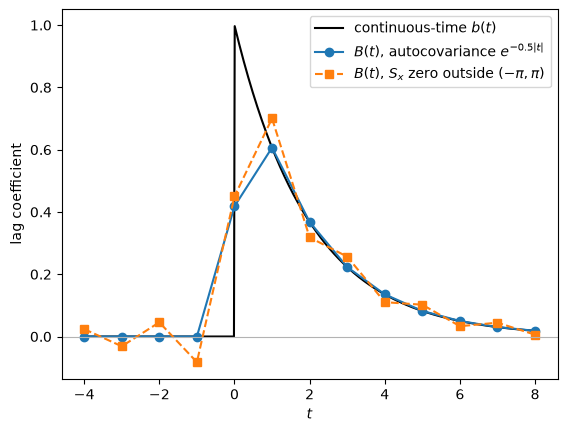
Fig. 24.2 Continuous-time lag and its sampled projections#
The coefficient \(B(0)\) at lag zero is between \(0.42\) and \(0.45\), while \(b(0) = 1\), because the sampled regression assigns to date zero an average of \(b\) over nearby dates.
When \(x\) has no power above frequency \(\pi\), the one-sided lag \(b\) projects onto a two-sided discrete lag with coefficients of alternating sign at negative \(t\).
An econometrician who tested whether the discrete-time lag distribution is one-sided, or who read \(B(0)\) as the instantaneous response, would draw wrong conclusions about \(b\) from a correctly estimated \(B\).
Exercise 24.1 derives the sign pattern.
24.4.3. Seasonal noise in regressors#
Sims [1974] studies the regression (24.7) when both variables contain seasonal noise.
He lets \(y = x * b + u\) and \(z = w * c + v\), where \(*\) denotes convolution, \(v\) is uncorrelated with \(w\), the seasonal noises \(z\) and \(w\) are uncorrelated with \(x\) and \(u\), and the econometrician observes \(y' = y + z\) and \(x' = x + w\).
The least squares regression of \(y'\) on all leads and lags of \(x'\) has the unconstrained lag distribution \(b'\) with
a weighted average of \(\tilde b\) and \(\tilde c\) whose weights vary with frequency.
When the noise in \(y\) is unrelated to the noise in \(x\), so that \(c = 0\), \(\tilde b'\) is close to \(\tilde b\) except at the seasonal frequencies, where \(S_w\) is large and \(\tilde b'\) falls toward zero.
Sims [1974] states the large-sample behavior of constrained least squares as his equation (2.7), crediting Sims [1972]: when we estimate the lag distribution “by least squares subject to prior constraints, the estimate \(\hat b\) will minimize, subject to the constraints, the quantity”
which is, up to the factor \(1/2\pi\) and an additive constant, (24.8) with \(S_{x'} = S_x + S_w\) in place of \(S_x\), \(\tilde b'\) in place of \(\tilde b\), and \(\hat b\) in place of \(d\).
The criterion puts heavy weight on fitting \(\tilde b'\) at the seasonal frequencies, where \(\tilde b'\) is most biased.
Sims draws the consequence:
because \(|\tilde{\hat b} - \tilde b'|^2\) at seasonal frequencies is given especially strong weight in the criterion function (2.7), constraints preventing sharp peaks or dips in \(\tilde{\hat b}\) at seasonals only result in estimates which have wide peaks or dips at seasonals, trading relatively more error at values away from the seasonal for a good fit very close to the seasonal.
Sims considers two true lag distributions: the identity lag, with \(b_0 = 1\) and \(b_s = 0\) for \(s \neq 0\), and the Koyck lag \(b_s = 0.9^s\) for \(s \geq 0\).
He sets the autocovariance function of \(x\) to \(0.9^{|t|}\).
The seasonal noise \(w\) is a moving average of white noise whose weights Sims gives in his footnote 6.
The weights are the convolution of a filter that averages five values four quarters apart with a filter that subtracts from each value the average of the sixteen surrounding quarters.
Sims scales \(w\) to have one-fourth the variance of \(x\).
The noise has peaks at the seasonal frequencies and no power at frequency zero.
# moving average weights of w, lags -16, ..., 16 (Sims 1974, footnote 6)
h1 = np.zeros(17)
h1[8 + 4 * np.arange(-2, 3)] = 1 / 5
h2 = -np.ones(17) / 16
h2[8] = 1.0
h_w = np.convolve(h1, h2)
h_w_ft = sum(h * np.exp(-1j * ω * k) for k, h in zip(range(-16, 17), h_w))

S_x74 = (1 - 0.9**2) * ar_spectrum(0.9)          # unit variance
S_w74 = np.abs(h_w_ft)**2
S_w74 = S_w74 * 0.25 / np.mean(S_w74)            # one-fourth the variance of x
S_xp74 = S_x74 + S_w74


def lag_from_ft(B_ft, t_vals):
    return np.array([np.mean(B_ft * np.exp(1j * ω * t)).real for t in t_vals])


t74 = np.arange(-8, 13)
b_identity_ft = np.ones(n_grid)
b_koyck_ft = 1 / (1 - 0.9 * z)
bp_identity = lag_from_ft(b_identity_ft * S_x74 / S_xp74, t74)
bp_koyck = lag_from_ft(b_koyck_ft * S_x74 / S_xp74, t74)
print(f"unconstrained coefficient at lag zero, identity lag: "
      f"{bp_identity[t74 == 0][0]:.2f}")
unconstrained coefficient at lag zero, identity lag: 0.63
fig, axes = plt.subplots(1, 2, figsize=(11, 4))
ax = axes[0]
ax.plot(ω[half], np.log(S_x74[half]), label="$S_x$")
ax.plot(ω[half], np.log(S_xp74[half]), label="$S_{x'} = S_x + S_w$")
ax.set_xticks(*π_ticks)
ax.set_xlabel(r"$\omega$")
ax.set_ylabel("log spectral density")
ax.legend()

ax = axes[1]
ax.plot([0], [1.0], "kx", ms=8, label="true identity lag at $t = 0$")
ax.plot(t74, bp_identity, "o-", label="estimated, identity lag")
koyck_t = t74[t74 >= 0]
ax.plot(koyck_t, 0.9**koyck_t, "k+", ms=10, label="true Koyck lag $0.9^t$")
ax.plot(t74, bp_koyck, "s-", label="estimated, Koyck lag")
ax.set_xticks(np.arange(-8, 13, 4))
ax.set_xlabel("$t$")
ax.set_ylabel("lag coefficient")
ax.legend(loc="lower center", bbox_to_anchor=(0.5, 1.0), ncol=2, fontsize=9,
          frameon=False)
plt.tight_layout()
plt.show()
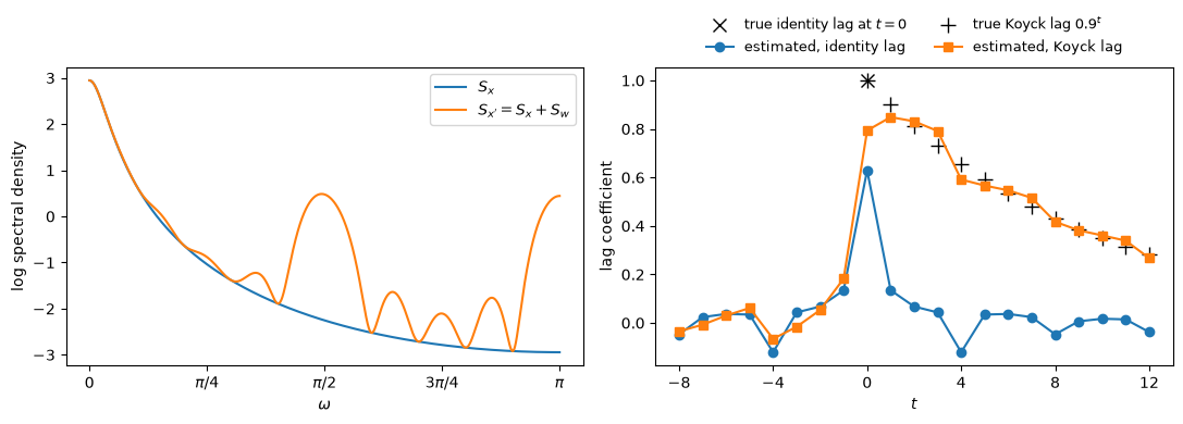
Fig. 24.3 Seasonal noise and estimated lag distributions#
The seasonal noise leaves the sum of the coefficients unbiased, because the noise has no power at frequency zero.
It lowers the coefficient at lag zero of the identity lag to about \(0.63\), and it adds seasonal ripples to both lag distributions, including coefficients on future values of \(x'\).
Two Illustrations of the Quantity Theory of Money uses the same argument: a component with no power at frequency zero leaves the sum of the lag coefficients \(h(0) = S_{yz}(0)/S_z(0)\) unchanged.
The function below solves the large-sample normal equations of a regression of \(y'\) on a set of lags of \(x'\) in the frequency domain.
Its optional argument weight multiplies the spectral density of \(x'\) and the cross spectrum of \(y'\) and \(x'\) by \(|\tilde k(\omega)|^2\), which is the effect of filtering both \(y'\) and \(x'\) by a filter \(k\); Exercise 24.2 uses it.
def constrained_lag(b_ft, lags, weight=None):
    """Large-sample least squares coefficients on x'(t - j), j in lags,
    for the true lag with Fourier transform b_ft and c = 0."""
    wt = np.ones(n_grid) if weight is None else weight
    M = np.array([[np.mean(wt * S_xp74 * np.cos(ω * (j - k))) for k in lags]
                  for j in lags])
    m = np.array([np.mean(wt * S_x74 * b_ft * np.exp(1j * ω * j)).real
                  for j in lags])
    return np.linalg.solve(M, m)


print("identity lag, x'(t) only:         ",
      np.round(constrained_lag(b_identity_ft, [0]), 3))
print("identity lag, x'(t) and x'(t - 1):",
      np.round(constrained_lag(b_identity_ft, [0, 1]), 3))
identity lag, x'(t) only:          [0.8]
identity lag, x'(t) and x'(t - 1): [0.576 0.336]
With only \(x'(t)\) as a regressor, the coefficient tends to \(0.80\), the attenuation factor \(1/(1 + 1/4)\) of the classical errors-in-variables model.
That coefficient is less biased than the unconstrained coefficient \(0.63\) at lag zero, but the sum of the coefficients, which the unconstrained regression estimates without bias, falls from \(1\) to \(0.80\).
Adding \(x'(t-1)\) gives coefficients that tend to \(0.58\) and \(0.34\), although the true lag distribution puts all its weight on date zero.
Sims [1974] reports \(0.80\), and \(0.58\) and \(0.31\).
Our computation, which follows his footnote 6 and formula (2.6), gives \(0.34\) for the second coefficient, and the other variants that we have tried give between \(0.33\) and \(0.34\).
He writes:
If these were estimates of, say, a short-run demand function for labor, the evidence for “short-run increasing returns to scale” would appear very strong, and by keeping the lag distribution short, evidence of the presence of seasonal bias would be suppressed.
His remedy is to filter both variables with the same filter \(k\), which he writes \(a\), that removes power near the seasonal frequencies.
Filtering both variables leaves the unconstrained lag distribution \(b'\) unchanged, and it replaces the weight \(S_{x'}\) in the constrained criterion by \(|\tilde k|^2 S_{x'}\).
Constrained least squares then fits \(\tilde b'\) at nonseasonal frequencies, where \(\tilde b'\) is close to \(\tilde b\).
Two Illustrations of the Quantity Theory of Money describes the opposite choice of filter.
Lucas’s two-sided moving average with parameter \(\beta\) concentrates the weight \(|\tilde k|^2 S_x\) near frequency zero.
A regression of one filtered series on the other with a single coefficient converges to the average of \(\tilde b\) weighted by \(|\tilde k|^2 S_x\), and that average approaches the sum \(\tilde b(0)\) of the lag coefficients as \(\beta \to 1\).
24.5. Seasonal adjustment in dynamic models#
24.5.1. Filtering in dynamic systems#
Sims [1993] points out that a complete dynamic system lacks the invariance of the regression of Distributed lags.
If \(y(t) = A * \varepsilon(t)\) is the moving average representation of a vector process and the econometrician uses the filtered data \(c * y\), the moving average operator becomes \(c * A\):
Thus in contrast to the result in the regression case – where \(b\) is unaffected by filtering – for a complete dynamic system the basic estimated parameter \(A\) is altered by filtering.
In a regression, the econometrician models only the conditional distribution of \(y\) given \(x\).
Filtering \(y\) and \(x\) by the same filter multiplies the cross spectrum and the spectrum of \(x\) by \(|\tilde c|^2\), so \(\tilde b = S_{yx}/S_x\) does not change.
In a dynamic system, the econometrician models the joint distribution of all the variables, whose spectral density matrix is \(\tilde A \tilde A^*\), and filtering replaces \(\tilde A\) by \(\tilde c \tilde A\).
The cross-equation restrictions of a rational expectations model tie the coefficients of agents’ decision rules to the parameters of the processes that agents forecast, and so they tie the parameters of preferences and technology to the whole operator \(A\).
Fitting an unfiltered model to filtered data therefore moves the estimates of those parameters.
Filtering the model as well would restore the invariance described in Misspecified autoregressions when the frequency response of the filter vanishes only at isolated frequencies, as Exercise 24.3 shows.
Sims’s econometrician instead treats the filtered data as if they were unadjusted.
Hansen and Sargent [1993] compare the operations of Misspecified autoregressions in terms of their criterion (24.4).
In the formulation that they attribute to Sims, the econometrician filters the data but not the model, so the spectral density \(F^a(\omega) = c(e^{-i\omega}) F(\omega) c(e^{i\omega})^\top\) of the filtered data replaces \(F(\omega)\), and \(G(\omega, \delta)\) stays as it was.
In ideal seasonal adjustment (24.6), the econometrician deletes the seasonal bands.
Hansen and Sargent state Sims’s argument for adjusted data in terms of the second term of (24.4):
The argument is that the term \(A_2(\delta) = (1/2\pi)\int_{-\pi}^{\pi} \operatorname{trace}[G(\omega, \delta)^{-1} F^a(\omega)] \, d\omega\) assigns the most weight to approximation error at frequencies at which \(F^a(\omega)\) [or \(F(\omega)\), if unadjusted data are used] is large. Since \(F(\omega)\) is large at precisely those frequencies where \(G(\omega, \delta)\) is most misspecified, the effects of misspecification on the estimates of the parameters of preferences and technologies will be diminished by weighting by \(F^a(\omega)\) rather than \(F(\omega)\).
They add in a footnote that seasonal adjustment has an efficiency cost: the overidentifying restrictions that a rational expectations model imposes across equations and across frequencies are most informative at the high-power seasonal frequencies that adjustment suppresses.
Sims [1993] describes the limit of an autoregression fitted to filtered data.
The limiting coefficients minimize a quadratic distance between the model’s one-step-ahead prediction filter and that of the filtered data, weighted by the spectral density of the filtered data.
Suppose that the parameterization can match the filtered data’s prediction filter closely outside the seasonal bands but cannot vary sharply over intervals as short as the bands, and that the bands are narrow.
Then, as adjustment drives the spectral density of the filtered data toward zero in the bands, the best-fitting filter fits well outside the bands and interpolates across them.
Sims shows that fitting a filter that is arbitrary in the bands to data with near-zero power there inflates the one-step-ahead forecast error by “one plus the ratio of the aggregate length of the seasonal bands to \(2\pi\).”
24.5.2. Hansen and Sargent’s experiment#
Hansen and Sargent [1993] study a linear-quadratic version of a stochastic growth model in which a planner chooses consumption, investment, and capital.
In the true model, the productivity parameter \(\gamma_{s(t)}\) varies periodically with the quarter \(s(t)\), taking the values \(0.13\), \(0.1\), \(0.1\), and \(0.08\); the adjustment cost parameter is \(\phi_1 = 0.3\); and the endowment shock \(d_t\) follows a first-order autoregression with coefficient \(0.4\).
The econometrician fits a model that is correct in all respects except that it has a constant productivity parameter \(\gamma\).
The econometrician imposes the true values of all the other parameters and estimates \(\gamma\), \(\phi_1\), and the coefficients \(a_1\), \(a_4\), and \(a_5\) of an autoregression for the endowment shock with lags \(1\), \(4\), and \(5\).
Hansen and Sargent apply (24.4) to the process that stacks the four observations of each year, so the mean \(\nu\) contains the four seasonal means.
A model with a constant \(\gamma\) implies the same mean in every quarter.
Their equation (4.11) writes the mean term as a sum over the frequencies \(0\), \(\pi/2\), \(\pi\), and \(3\pi/2\) of the Fourier components of the errors in the seasonal means, each divided by the model’s spectral density of \(y_t\) at that frequency.
Hansen and Sargent compare three kinds of data:
unadjusted data, for which the criterion is (24.4);
data from which the econometrician has removed seasonal means by regressing on seasonal dummies, for which the criterion drops the mean term of (24.4); and
ideally adjusted data, for which the criterion deletes the seasonal bands from the first two terms and drops the mean term.
Their Table 1 reports the minimizers of the three criteria:
parameter |
seasonally unadjusted |
seasonal means removed |
seasonally adjusted |
truth |
|---|---|---|---|---|
\(\gamma\) |
0.0996 |
0.1030 |
0.1025 |
\(\gamma_{s(t)}\) |
\(\phi_1\) |
0.4132 |
0.2854 |
0.3007 |
0.3000 |
\(a_1\) |
0.931 |
0.3250 |
0.3987 |
0.4000 |
\(a_4\) |
0.4383 |
0.1598 |
−0.0003 |
0.000 |
\(a_5\) |
−0.4298 |
−0.1261 |
−0.0005 |
0.000 |
With unadjusted data, the estimates of \(a_1\), \(a_4\), and \(a_5\) put into the endowment process the seasonality that periodic productivity generates, and the estimate of \(\phi_1\) overstates the adjustment cost.
With seasonal means removed, the estimates of \(a_4\) and \(a_5\) still put some seasonality into the endowment process, and the estimates of \(\phi_1\) and \(a_1\) fall below the truth.
Hansen and Sargent explain the estimates from data with seasonal means removed, where \(c_t\) and \(i_t\) are consumption and investment:
In order to diminish the errors at the seasonal bands, the estimates put some seasonality into \(\{c_t, i_t\}\) the only way that the model permits, namely, through the endowment process. Doing that helps the model ‘match’ at the seasonal frequencies at the cost of worse fit at the nonseasonal frequencies.
Hansen and Sargent attribute the larger errors with unadjusted data, compared with data with seasonal means removed, to the mean term.
The model can shrink that term only by raising its spectral density at the seasonal frequencies, which the larger estimates of \(a_4\) and \(a_5\) do.
With ideally adjusted data, the estimates of \(\phi_1\) and of the endowment process are close to the truth, and the estimate \(0.1025\) of \(\gamma\) equals the average \((0.13 + 0.1 + 0.1 + 0.08)/4\) of the quarterly productivity parameters.
24.5.3. Sims’s permanent income examples#
Sims [1993] uses a permanent income model to give one example in which adjusted data reduce the error and one in which they increase it.
A consumer with quadratic utility and discount factor \(\beta\) faces a gross interest rate \(\beta^{-1}\), so that consumption \(C_t\) is a martingale and
where \(Y_t\) is income.
Income is the sum \(Y_t = Y^N_t + Y^S_t\) of a nonseasonal component
normalized to have unit variance, and a deterministic seasonal component that repeats the pattern \(\sqrt{2}, 0, -\sqrt{2}, 0\).
The deterministic seasonal is perfectly predictable, so it never revises expected income and does not affect \(\Delta C_t\).
If \(Y^N_t = \psi(L) \varepsilon_t\), then \(\Delta C_t = (1 - \beta)\psi(\beta) \varepsilon_t\), and the coefficient of a regression of the income innovation \(\varepsilon_t\) on \(\Delta C_t\) is \(1/[(1 - \beta)\psi(\beta)]\).
The LQ Permanent Income Model derives this formula as (92.15), with \(d\) in place of \(\psi\).
Sims does not state \(\beta\); we use \(\beta = 0.95\), the value implied by his coefficient of \(20\) in his second example below.
With \(\psi(L) = (1 - 0.9L)^{-2}\), the coefficient is \((1 - 0.9\beta)^2 / (1 - \beta) = 0.4205\), the value that Sims reports.
An econometrician who fits an autoregression \(a(L) Y_t = e_t\) to income and believes the permanent income model computes the coefficient \(a(\beta)/(1 - \beta)\).
Sims first supposes that the econometrician fits a ninth-order autoregression to unadjusted data, with no seasonal dummies.
The large-sample autoregression is the m-projection of the income process onto the ninth-order autoregressions, so it solves the Yule–Walker equations with the autocovariances \(R^N(s) + R^S(s)\), where \(R^N\) is the autocovariance function of \(Y^N\) and \(R^S(s) = \cos(\pi s/2)\) is that of the seasonal pattern.
β = 0.95
fN_ar2 = ar_spectrum([1.8, -0.81])
fN_ar2 = fN_ar2 / np.mean(fN_ar2)                    # unit variance


def seasonal_autocov(n_lags, gain2=1.0):
    """R^S(s) = cos(π s / 2), times the squared gain of a filter at π/2."""
    return gain2 * np.cos(np.pi * np.arange(n_lags + 1) / 2)


def implied_coefficient(a):
    """Coefficient of ε on ΔC implied by the autoregression a(L) Y = e."""
    a_β = 1 - sum(a_j * β**(j + 1) for j, a_j in enumerate(a))
    return a_β / (1 - β)


a9 = yule_walker(autocov(fN_ar2, 9) + seasonal_autocov(9), 9)
print("AR(9) coefficients:", np.round(a9, 4))
print(f"true coefficient {(1 - 0.9 * β)**2 / (1 - β):.4f}, "
      f"implied by the AR(9): {implied_coefficient(a9):.4f}")
AR(9) coefficients: [ 1.792  -1.1156  0.5775  0.0464 -0.5775 -0.0464  0.5775 -0.2084 -0.059 ]
true coefficient 0.4205, implied by the AR(9): 0.4925
Our projection gives the coefficients of Sims’s equation (17), except for the coefficient on \(Y_{t-8}\): we obtain \(-0.2084\), and Sims prints \(+0.2084\).
Only the negative sign reproduces his implied coefficient of \(0.4925\), a bias factor of \(1.17\).
The ninth-order autoregression forecasts most of the deterministic seasonal, but it attributes part of the innovation in income to a stochastic seasonal component, and the permanent income model then implies that consumption responds less to an income innovation than it actually does.
Sims observes that the regression of the autoregression’s forecast errors on \(\Delta C_t\) in the data still recovers \(0.4205\).
The autoregression’s forecast error is the true innovation plus a component orthogonal to it, and \(\Delta C_t\) is proportional to the true innovation.
An econometrician who used the ninth-order autoregression would therefore conclude, wrongly, that consumption reacts to income more strongly than the theory implies.
Sims next adjusts both \(C\) and \(Y\) by subtracting the seasonal component that the filter \(\kappa(L)\kappa(L^{-1})\) extracts, where
is the filter that he writes \(F(L)\), and he treats the adjusted series as if they were unadjusted data.
The adjusted data have spectral density \((1 - |\kappa(e^{-i\omega})|^2)^2\) times that of the unadjusted data.
Sims reports that a second-order autoregression fitted to adjusted income gives a bias factor of only \(1.0137\).
With the filter as we read it, we obtain a bias factor of \(0.893\) for that computation, and other readings that we tried do not reproduce \(1.0137\) either; the same reading gives \(17.08\) for his second example below, within \(0.02\) of his \(17.06\).
We add a computation that Sims does not report: deleting the seasonal bands from the criterion and fitting a second-order autoregression recovers the truth, because \(Y^N\) is a second-order autoregression and the deterministic seasonal has all its power at frequency \(\pi/2\).
κ_ft = (0.25 * sum(z**(4 * k) for k in range(4))
        - 0.0625 * sum(z**k for k in range(16)))
adjust2 = (1 - np.abs(κ_ft)**2)**2                # squared gain of 1 - κκ*
z_q = np.exp(-1j * np.pi / 2)                     # the seasonal frequency π/2
κ_q = (0.25 * sum(z_q**(4 * k) for k in range(4))
       - 0.0625 * sum(z_q**k for k in range(16)))
gain2_q = (1 - np.abs(κ_q)**2)**2                 # zero: the seasonal is removed

a2_adj = yule_walker(autocov(fN_ar2 * adjust2, 2)
                     + seasonal_autocov(2, gain2_q), 2)
print(f"AR(2), adjusted data: implied coefficient "
      f"{implied_coefficient(a2_adj):.4f}, bias factor "
      f"{implied_coefficient(a2_adj) / 0.4205:.3f}")

keep_B = seasonal_keep(np.pi / 8)
a2_B, _ = ar_projection(fN_ar2, 2, keep_B)       # the seasonal lies in a deleted band
print("AR(2), seasonal bands deleted:", np.round(a2_B, 4),
      f" implied coefficient {implied_coefficient(a2_B):.4f}")
AR(2), adjusted data: implied coefficient 0.3755, bias factor 0.893
AR(2), seasonal bands deleted: [ 1.8  -0.81]  implied coefficient 0.4205
In Sims’s second example, an econometrician who uses adjusted data does worse than one who uses unadjusted data.
Sims replaces \(Y^N\) by unit-variance white noise, for which the true coefficient is \(1/(1 - \beta) = 20\), and he reports that a ninth-order autoregression fitted to unadjusted data implies a coefficient of \(20.62\) and that adjusted data imply \(17.06\).
Sims does not state the order of the autoregression that he fits to adjusted data in this example; we fit a second-order autoregression, as in his first example, and also report a ninth-order autoregression.
f_white = np.ones(n_grid)
a9_w = yule_walker(autocov(f_white, 9) + seasonal_autocov(9), 9)
a2_adj_w = yule_walker(autocov(f_white * adjust2, 2)
                       + seasonal_autocov(2, gain2_q), 2)
a9_adj_w = yule_walker(autocov(f_white * adjust2, 9)
                       + seasonal_autocov(9, gain2_q), 9)
a2_band_w, _ = ar_projection(f_white, 2, keep_B)
print(f"true coefficient:                   {1 / (1 - β):.2f}")
print(f"AR(9), unadjusted data:             {implied_coefficient(a9_w):.2f}")
print(f"AR(2), data adjusted with κκ*:      {implied_coefficient(a2_adj_w):.2f}")
print(f"AR(9), data adjusted with κκ*:      {implied_coefficient(a9_adj_w):.2f}")
print(f"AR(2), seasonal bands deleted:      {implied_coefficient(a2_band_w):.2f}")
γ_adj = autocov(f_white * adjust2, 4)
print("autocorrelations of adjusted white noise, lags 1 to 4:",
      np.round(γ_adj[1:] / γ_adj[0], 3))
print("AR(2) coefficients, adjusted data:", np.round(a2_adj_w, 3))
true coefficient:                   20.00
AR(9), unadjusted data:             20.64
AR(2), data adjusted with κκ*:      17.08
AR(9), data adjusted with κκ*:      16.82
AR(2), seasonal bands deleted:      20.00
autocorrelations of adjusted white noise, lags 1 to 4: [ 0.082  0.088  0.096 -0.219]
AR(2) coefficients, adjusted data: [0.076 0.082]
Our computation gives \(20.64\) for unadjusted data, close to Sims’s \(20.62\).
Sims’s adjustment filter removes the seasonal, but it also reduces the spectral density of the data in neighborhoods of the seasonal frequencies, so the econometrician fits the second-order autoregression to a process whose spectral density has dips that white noise does not have.
Adjusted white noise has positive autocorrelations, between \(0.08\) and \(0.10\) at lags 1 to 3, so the second-order autoregression has positive coefficients, \(0.076\) and \(0.082\), and \(a(\beta) = 0.854\).
The econometrician attributes persistence to income innovations that have none, and infers that consumption responds more to an income innovation than it does.
Deleting the seasonal bands from the criterion leaves the other frequencies unchanged, and the second-order autoregression fitted outside the bands has coefficients equal to zero, which imply the true coefficient \(20\).
In Exercise 24.3, the econometrician filters the model as well as the data.
Sims concludes:
Use of unadjusted data and a correctly specified model of seasonal variation is always the best option. But treating seasonality casually, as a ‘nuisance’ component of the model, can lead to worse errors than those produced by use of adjusted data.
24.6. Garbling and the data processing inequality#
Blackwell’s Theorem on Comparing Experiments calls an experiment a garbling of another experiment when its signal can be generated from the other experiment’s signal by a Markov kernel.
The data processing inequality says that applying the same Markov kernel to two distributions cannot increase any f-divergence between them, including the KL divergence, and that the divergence is unchanged when the kernel is induced by a sufficient statistic for the pair.
Filtering, deleting frequency bands, removing seasonal means, and sampling are garblings, and the inequality organizes what this lecture has found about them.
24.6.1. Filters, frequency bands, and the data processing inequality#
When an econometrician filters the data by \(c(L)\) and filters the model in the same way, the filtered series is the same function of the unfiltered series under the true process and under the model.
Filtering therefore applies one Markov kernel, a deterministic one, to both processes, and the data processing inequality says that filtering cannot increase the divergence between them.
When the frequency response \(c(e^{-i\omega})\) is zero at most at isolated frequencies, filtering multiplies \(f\) and \(g\) by \(|c(e^{-i\omega})|^2\) and leaves the ratio \(f/g\) unchanged at every other frequency, so the divergence rate (24.2) does not change.
A filter applied to both the data and the model whose frequency response is zero at most at isolated frequencies leaves the divergence rate and the m-projection unchanged, however much it shrinks the spectral densities near those frequencies.
If, in addition, the spectral measure of the data puts no mass at those frequencies, the filtered series determines the unfiltered series in mean square, so the filter is a sufficient statistic for the pair, and the invariance of Misspecified autoregressions is the equality case of the data processing inequality.
Sims’s filter \(1 - \kappa(L)\kappa(L^{-1})\) is zero at \(\pm\pi/2\), at \(\pi\), and at two frequencies near \(\pm 0.485\pi\).
It removes the deterministic seasonal, whose spectral measure puts all its mass at \(\pm\pi/2\), and the equality applies to what remains, as Exercise 24.3 shows.
A filter cannot delete a band of frequencies from the likelihood.
A filter whose frequency response is zero on a band makes the filtered processes linearly deterministic, and formula (24.2), which assumes spectral densities bounded away from zero, no longer applies.
For example, if the true process and the model are white noise with variances \(1\) and \(2\), the filtered model is \(\sqrt{2}\) times the filtered true process, so the divergence between the distributions of \(T\) filtered observations equals the divergence between the distributions of \(T\) unfiltered observations at every \(T\).
Hansen and Sargent define ideal seasonal adjustment in the frequency domain instead, by omitting the seasonal frequencies from the frequency-domain likelihood.
The finite Fourier transforms \(w_j\) at the frequencies \(\omega_j = 2\pi j / T\), \(j = 0, \ldots, T - 1\), are an invertible linear transformation of the sample, so dropping the transforms at the frequencies in the bands is a garbling at every sample size.
Divided by \(T\), the divergence between the distributions of the remaining transforms converges to the divergence rate restricted to the set \(K\) of frequencies outside the bands:
Twice \(D_K\) is the first term of (24.6) minus terms that do not depend on \(\delta\), so the statement after (24.6) that the restricted rate is at most the full rate is the data processing inequality.
Equality holds when \(f = g\) almost everywhere in the bands: then, in large samples, the transforms in the bands have the same distribution under the two processes and are independent of the remaining transforms, so dropping them discards nothing that distinguishes the processes.
Filtering the data but not the model, as Sims’s econometrician does, applies the kernel to only one of the two distributions, and the data processing inequality says nothing about it.
Sims’s permanent income examples go in opposite directions, although each comparison also changes the order of the autoregression.
In the first, adjusted data bring the bias factor closer to one: it is \(1.17\) for a ninth-order autoregression fitted to unadjusted data, and \(0.893\) by our computation and \(1.0137\) by Sims’s for a second-order autoregression fitted to adjusted data.
In the second, adjusted data move the implied coefficient from \(20.64\) to \(17.08\) with a second-order autoregression, or to \(16.82\) with a ninth-order one, farther from the true value \(20\).
24.6.2. A Blackwell chain#
Hansen and Sargent’s three kinds of data are ordered by garbling.
Data from which seasonal means have been removed are the residuals from a regression of the unadjusted data on seasonal dummies, so they are a function of the unadjusted data.
Ideally adjusted data are a function of the data with seasonal means removed.
When \(T\) is a multiple of \(4\), the seasonal dummies span the same space as the finite Fourier vectors at the frequencies \(0\), \(\pi/2\), \(\pi\), and \(3\pi/2\), so removing seasonal means drops the transforms at those four frequencies, and ideal adjustment drops, in addition, the transforms in the bands around \(\pi/2\), \(\pi\), and \(3\pi/2\).
The three kinds of data are nested sets of Fourier transforms, and each is a garbling of the one before it at every sample size.
For each \(\delta\), subtracting from each of the three criteria the terms that do not depend on \(\delta\) leaves twice the divergence rate between the true process and the model at \(\delta\) after the corresponding garbling.
So at every \(\delta\), the divergence falls weakly from the first kind of data to the second and from the second to the third.
The minimized divergence falls too: if \(\delta^*\) minimizes the divergence for the finer data, the minimum for the coarser data is at most the coarser divergence at \(\delta^*\), which is at most the finer divergence at \(\delta^*\).
In Hansen and Sargent’s Table 1, the errors in the probability limits of the estimates also fall at every step.
We measure the error in \(\gamma\) from the average \(0.1025\) of the quarterly productivity parameters.
table_1 = {"γ": (0.0996, 0.1030, 0.1025), "φ_1": (0.4132, 0.2854, 0.3007),
           "a_1": (0.931, 0.3250, 0.3987), "a_4": (0.4383, 0.1598, -0.0003),
           "a_5": (-0.4298, -0.1261, -0.0005)}
true_values = {"γ": np.mean([0.13, 0.1, 0.1, 0.08]), "φ_1": 0.3, "a_1": 0.4,
               "a_4": 0.0, "a_5": 0.0}
print("absolute errors   unadjusted   means removed   ideally adjusted")
for name, estimates in table_1.items():
    errors = np.abs(np.array(estimates) - true_values[name])
    print(f"{name:>15}" + "".join(f"{e:15.4f}" for e in errors))
absolute errors   unadjusted   means removed   ideally adjusted
              γ         0.0029         0.0005         0.0000
            φ_1         0.1132         0.0146         0.0007
            a_1         0.5310         0.0750         0.0013
            a_4         0.4383         0.1598         0.0003
            a_5         0.4298         0.1261         0.0005
Blackwell’s theorem says that a decision maker who knows the likelihoods of an experiment can do at least as well with it as with any garbling of it, in every decision problem.
Sims’s conclusion, “Use of unadjusted data and a correctly specified model of seasonal variation is always the best option,” is the counterpart of that theorem for estimation: with a correctly specified model, deleting frequencies cannot lower the asymptotic variance of the maximum likelihood estimator.
Hansen and Sargent’s Table 1 reverses Blackwell’s ranking.
Their econometrician evaluates the three kinds of data with the likelihoods of a misspecified model, so Blackwell’s theorem does not apply, and the probability limits of the estimates of the parameters of preferences, technology, and the endowment process are closest to the truth for the coarsest data.
Hansen and Sargent’s introduction describes the argument that their reversal answers:
Other writers had asserted that seasonally unadjusted data ought to be used to estimate rational expectations models, on the grounds that the agents being modelled were themselves assumed to be solving forecasting and signal extraction problems using seasonally unadjusted data, and that the cross-equation restrictions implied by their behavior applied to seasonally unadjusted series. Sims responded that that argument assumes that the model is correctly specified, and asserted that admitting the possibility of approximation error would alter the situation.
The other writers are Sargent [1978] and Singleton [1988].
The agents inside the model know the true likelihoods, so Blackwell’s theorem applies to them, and they have no reason to garble their data.
Sims’s reply is that the theorem does not apply to an econometrician whose model is misspecified.
Incentives for Information Transfer describes a different reason that a decision maker can prefer a garbled experiment.
24.6.3. Two pairs of distributions#
The data processing inequality applies to any two distributions.
Applied to the true process and the model at \(\delta\), it says that a garbling cannot increase the misspecification; Hansen and Sargent’s ideal adjustment, their version of Sims’s argument, uses this side.
Applied to the model at two parameter values \(\delta\) and \(\delta'\), it says that a garbling cannot make them easier to tell apart.
If a garbling maps them to the same distribution, they become observationally equivalent, which is what Hansen and Sargent mean when they write that omitting frequencies “might hinder identification by introducing additional minimizers.”
For nearby parameter values, the divergence is one half a quadratic form in the Fisher information matrix, as in Exponential Family and Maximum Entropy.
For a scalar model with spectral density \(g(\omega; \delta)\) fitted to the frequencies in a set \(K\), the Fisher information matrix of the frequency-domain likelihood is
so deleting frequencies lowers it in the matrix order: \(\mathcal{I}_K(\delta) \preceq \mathcal{I}(\delta)\), where \(\mathcal{I}\) uses all frequencies.
This is the Fisher-information form of the data processing inequality in Blackwell’s Theorem on Comparing Experiments.
Inversion reverses the matrix order, so with a correctly specified model, \(\sqrt{T}\) times the estimator’s error has asymptotic covariance matrix \(\mathcal{I}_K(\delta)^{-1} \succeq \mathcal{I}(\delta)^{-1}\), which is the efficiency cost in Hansen and Sargent’s footnote 11.
The two matrices are equal when \(\nabla_\delta \log g = 0\) almost everywhere on the deleted frequencies, so that those frequencies carry no information about \(\delta\).
Hansen and Sargent’s correctly specified examples remain identified when the seasonal frequencies are dropped, although the parameters “impinge most strongly on the seasonal frequencies”:
they affect all frequencies in ways that are sufficient to preserve their identification even when the seasonal frequencies are dropped.
There, deleting the bands lowers the information about the parameters without making any other parameter value observationally equivalent to the true one.
Hansen and Sargent’s concluding remarks set the two sides of the inequality against each other:
Second, when one is estimating a correctly specified model, there will occur a substantial efficiency loss from using seasonally adjusted data, a loss that grows with the importance of the seasonality in the raw data. In practice, there can be a trade-off between variance and bias of estimators, the dimensions of which we have not explored in this paper.
Their footnote 17 adds: “On the basis of the logic leading to (4.2), something can be said about the asymptotic distributions of estimators of misspecified models. We plan to explore this in subsequent work.”
When the data come from a Gaussian process whose spectral density \(f\) differs from \(g(\cdot\,; \delta^*_K)\), where \(\delta^*_K\) is the m-projection over the frequencies in \(K\), \(\sqrt{T}(\hat \delta_K - \delta^*_K)\) has asymptotic covariance matrix \(\mathcal{H}_K^{-1} \mathcal{J}_K \mathcal{H}_K^{-1}\), where
with \(g\) and its derivatives evaluated at \(\delta^*_K\).
\(\mathcal{H}_K\) is the Hessian of the divergence rate restricted to \(K\), and \(\mathcal{J}_K\) is the asymptotic variance of the score of (24.5) divided by \(\sqrt{T}\).
The factor \((f/g)^2\) comes from the variance of the periodogram, which stays near \(f^2\).
When \(f = g(\cdot\,; \delta^*_K)\), both matrices equal \(\mathcal{I}_K\), and the covariance matrix reduces to \(\mathcal{I}_K^{-1}\).
The code below computes, for the seasonal example, the AR(1) projection with bands of several widths deleted, the minimized divergence, and the asymptotic variance of \(\hat\rho\) in two cases: when the data come from \(x_t\) alone, so that the AR(1) is correct, and when they come from \(y_t = x_t + s_t\).
def ar1_derivatives(ρ, σ2):
    """∇ log g and ∇² log g on the grid for g = σ²/|1 - ρe^{-iω}|², θ = (ρ, σ²)."""
    d1 = np.vstack([2 * np.real(z / (1 - ρ * z)), np.ones(n_grid) / σ2])
    d2 = np.zeros((2, 2, n_grid))
    d2[0, 0] = 2 * np.real(z**2 / (1 - ρ * z)**2)
    d2[1, 1] = -1 / σ2**2
    return d1, d2


def ar1_covariance(f, ρ, σ2, keep):
    """Asymptotic covariance matrix of √T(θ̂ - θ*), formula (ae_sandwich)."""
    d1, d2 = ar1_derivatives(ρ, σ2)
    r = np.where(keep, f / ar_spectrum(ρ, σ2), 0.0)
    H = 0.5 * ((d1 * r) @ d1.T
               + (d2 * np.where(keep, 1 - r, 0.0)).sum(axis=2)) / n_grid
    J = 0.5 * ((d1 * r**2) @ d1.T) / n_grid
    H_inv = np.linalg.inv(H)
    return H_inv @ J @ H_inv


print("band width     ρ*    divergence   Var, x alone   Var, y = x + s")
for Δ in (0, np.pi / 16, np.pi / 8, np.pi / 4, np.pi / 2):
    keep = seasonal_keep(Δ)
    a_K, σ2_K = ar_projection(f_y, 1, keep)
    V_x = ar1_covariance(f_x, ρ_x, 1.0, keep)[0, 0]
    V_y = ar1_covariance(f_y, a_K[0], σ2_K, keep)[0, 0]
    print(f"{Δ / np.pi:9.4f}π {a_K[0]:7.4f} "
          f"{kl_rate(f_y, ar_spectrum(a_K, σ2_K), keep):11.5f} "
          f"{V_x:13.4f} {V_y:15.4f}")
band width     ρ*    divergence   Var, x alone   Var, y = x + s
   0.0000π  0.6200     0.42909        0.1900          4.5736
   0.0625π  0.8520     0.04467        0.1919          0.4278
   0.1250π  0.8733     0.01241        0.1944          0.3125
   0.2500π  0.8850     0.00309        0.2017          0.2692
   0.5000π  0.8998     0.00000        0.2642          0.2655
With bands of width \(\pi/2\), only the frequencies below \(\pi/4\) remain.
When the AR(1) is correct, deleting bands of width \(\pi/8\) raises the asymptotic variance of \(\hat\rho\) from \(0.190\) to \(0.194\), about 2 percent, because the information about \(\rho\) is concentrated at low frequencies.
Hansen and Sargent’s footnote 11 describes rational expectations models differently: their cross-equation restrictions put much of the information at the high-power seasonal frequencies, where deleting bands costs more.
In the seasonal example, the estimator that uses all frequencies has asymptotic variance \(4.57\), 24 times the variance when the AR(1) is correct.
The periodogram ordinates at the seasonal peaks, where \(f/g\) is large, enter \(\mathcal{J}_K\) with the weight \((f/g)^2\).
Deleting bands of width \(\pi/8\) removes those ordinates and lowers the variance to \(0.31\), so here deleting bands lowers the variance as well as the bias.
The efficiency cost of deleting frequencies is guaranteed only for correctly specified models.
Exercise 24.4 finds the band width that balances bias against variance when the seasonal component is small.
Specification Tests builds a test that compares the band-deleted and full-band estimators and uses (24.13) to compute the variance of their difference when the model is misspecified.
24.6.4. Divergences, not estimates#
The data processing inequality bounds divergences; it does not say where the minimizer goes.
Deleting a band of low frequencies instead of the seasonal bands is also a garbling.
dist_0 = np.minimum(ω, 2 * np.pi - ω)
print(f"all frequencies:                 ρ* = {a_full[0]:.4f},  "
      f"divergence {kl_rate(f_y, g_full):.4f}")
for Δ in (np.pi / 8, np.pi / 4):
    keep_low = dist_0 >= Δ / 2              # delete a band of width Δ around zero
    a_low, σ2_low = ar_projection(f_y, 1, keep_low)
    print(f"low band of width {Δ / np.pi:.3f}π deleted: ρ* = {a_low[0]:.4f},  "
          f"divergence {kl_rate(f_y, ar_spectrum(a_low, σ2_low), keep_low):.4f}")
all frequencies:                 ρ* = 0.6200,  divergence 0.4291
low band of width 0.125π deleted: ρ* = 0.2459,  divergence 0.3660
low band of width 0.250π deleted: ρ* = 0.0168,  divergence 0.3298
The minimized divergence falls from \(0.429\) to \(0.366\) and \(0.330\), as the inequality requires, but \(\rho^*\) falls from \(0.62\) to \(0.25\) and \(0.02\), farther from the coefficient \(0.9\) of the nonseasonal component.
This garbling discards frequencies at which the seasonal component has almost no power and at which most of the information about \(\rho\) lies: a band of width \(\pi/8\) around zero holds 0.03 percent of the variance of \(s_t\) and 91 percent of \(\mathcal{I}(\rho)\) when the AR(1) is correct.
A garbling can improve the estimates of the parameters that an econometrician cares about when it discards the frequencies at which the model is wrong and keeps the frequencies that carry information about those parameters.
Hansen and Sargent’s third qualification in their concluding remarks allows for this: “it is undoubtedly true that particular examples of estimation of misspecified models can go against Sims’s recommendation.”
Their condition for ideal adjustment to work describes a garbling that discards exactly the misspecification.
If, for some \(\delta_0\), the model matches \(F\) outside the seasonal bands and matches the mean, then the garbling maps the true process and the model at \(\delta_0\) to the same distribution, because two Gaussian processes with the same mean and spectral density are the same process.
The garbled divergence at \(\delta_0\) is then zero, its smallest possible value.
Hansen and Sargent’s footnote 12 on measurement error fits the same reading:
Strictly speaking, to avail ourselves of such an argument that consistency can be retained by ignoring seasonal frequencies, it is necessary to assume that the measurement error is purely seasonal. Such a measurement error process would be linearly deterministic, i.e., perfectly predictable linearly from its own past.
For deleting the bands to remove a measurement error completely, the error’s spectral density must be zero outside the bands.
The integral of the logarithm of that spectral density is then \(-\infty\), and Kolmogorov’s formula of Misspecified autoregressions gives a one-step-ahead forecast error variance \(\sigma^2_\infty = 0\).
24.6.5. Low-frequency filters#
Hansen and Sargent end their paper by extending the argument to other filters:
Formally, the same arguments that support the use of seasonally adjusted data also apply to using data that have been filtered to eliminate, say, low-frequency components. For example, Hodrick and Prescott (1980) compose what is essentially a high-pass filter that eliminates very-low-frequency components from time series while leaving business cycle and higher frequencies intact. Prescott and many other researchers have tried to match data that have been filtered with the Hodrick–Prescott filter to theoretical models that they have designed explicitly to capture business cycle frequencies, but whose low-frequency properties they distrust. Such an empirical strategy can probably be rationalized through an appropriate application of our approximation criterion (4.2).
The cyclical component of the filter of Hodrick and Prescott [1997] with smoothing parameter \(\lambda\) has frequency response
which is zero only at \(\omega = 0\).
Because \(h(0) = 0\), the filter removes the mean, and the mean term of (24.3) drops out; because \(h\) is zero at no other frequency, filtering both the data and the model leaves the rest of the divergence rate unchanged.
For the stationary processes of this lecture, Gaussian maximum likelihood estimates of a model fitted to Hodrick–Prescott filtered data, with the model’s spectral density filtered in the same way, therefore converge to the same m-projection as estimates from unfiltered data with the mean term dropped.
In large samples, the filter can change what an econometrician estimates in three ways:
it can be applied to the data but not to the model, as in Sims’s formulation;
it can be replaced by the deletion of a band of low frequencies from the frequency-domain likelihood, a garbling that can improve the estimates when the model is wrong mainly at low frequencies, which is the case that Hansen and Sargent describe; or
it can be used with a criterion that is not a likelihood, such as the distance between a few variances and covariances of the filtered data and of the filtered model, in which the frequency response of the filter weights the frequencies.
The code below uses the smoothing parameter \(\lambda = 1600\) that is customary for quarterly data.
λ = 1600
h_hp = 4 * λ * (1 - np.cos(ω))**2 / (1 + 4 * λ * (1 - np.cos(ω))**2)
print(f"D(f || g) = {kl_rate(f_y, g_full):.6f},  "
      f"D(h²f || h²g) = {kl_rate(h_hp**2 * f_y, h_hp**2 * g_full):.6f}")
a_hp, _ = ar_projection(h_hp**2 * f_y, 1)
print(f"AR(1) projection of filtered data, unfiltered model: ρ* = {a_hp[0]:.4f}")
D(f || g) = 0.429093,  D(h²f || h²g) = 0.429093
AR(1) projection of filtered data, unfiltered model: ρ* = 0.1625
In the seasonal example, fitting an unfiltered AR(1) to filtered data gives \(\rho^* = 0.16\), because the filter removes the low-frequency power that pulls the projection toward \(0.9\).
24.6.6. Sampling#
Sampling a continuous-time process at integer dates is also a garbling: the sampled series is a function of the continuous-time path, under the true process and under the model alike.
So is the averaging over unit intervals that Sims uses in column (4) of his Table I.
The denominator of (24.9), the spectral density of the sampled regressor, shows the garbling in the frequency domain: sampling adds to frequency \(\omega\) the contributions of the frequencies \(\omega + 2\pi k\).
Applied to two continuous-time models, the data processing inequality says that sampling cannot make them easier to tell apart.
Two continuous-time processes whose spectral densities fold to the same discrete-time spectral density are observationally equivalent from sampled data, and in Sims’s setting, distinct continuous-time lag distributions can have the same discrete-time lag distribution \(B\).
An econometrician who reads \(B\) as \(b\) faces this identification problem.
Hansen and Sargent [1983] describe it:
It is a well known result from the theory of continuous time, covariance stationary stochastic processes that the continuous time spectral density function cannot, in general, be inferred from equispaced discrete time observations. This identification problem is commonly referred to as the aliasing phenomenon.
They show that restricting the continuous-time spectral density matrix to be rational “goes a significantly greater distance towards resolving the aliasing problem than has heretofore been recognized.”
Within the class of models with rational spectral densities, in general only a finite number of continuous-time models are observationally equivalent, in some regions of the parameter space “there may be no identification problem at all,” and for a first-order vector Markov process “there generally exists a discrete sampling interval sufficiently fine that the continuous time model is identified.”
Sampling is not one-to-one on the set of all continuous-time processes, but it can be one-to-one on a restricted family.
Hansen and Sargent add that the restrictions that economic theory imposes can also serve to identify the continuous-time model.
24.7. Concluding remarks#
The maximum likelihood estimator of a misspecified time series model converges to the m-projection of the true process onto the model.
The KL divergence rate (24.2) charges each frequency according to the ratio of the data’s spectral density to the model’s; in a distributed-lag regression, the spectral density of the regressor weights the error in the lag distribution at each frequency, as in (24.8).
A first-order autoregression fitted to a series whose nonseasonal component has coefficient \(0.9\) and whose seasonal component has one quarter of the variance of the nonseasonal component has \(\rho^* = 0.62\); deleting seasonal bands of width \(\pi/8\) raises \(\rho^*\) to \(0.87\).
Filtering the data and the model with the same invertible filter leaves the projection unchanged; deleting frequency bands, or filtering the data alone, changes it.
In the example of Sims [1971], least squares on sampled data puts a coefficient of about \(0.43\) at lag zero, where the continuous-time lag distribution has \(1\).
In the example of Sims [1974], seasonal noise in the regressor, together with a constraint that keeps the estimated lag distribution short, produces coefficients that, read as a short-run demand function for labor, would suggest short-run increasing returns to scale.
In the first example of Sims [1993], a misspecified seasonal model of unadjusted data understates the response of consumption to income by a factor of \(1.17\); in his second example, adjusted data produce a larger error than unadjusted data.
Optimal Misspecified Beliefs describes an equilibrium in which agents’ beliefs are the m-projection, in the sense of (24.4), of the process that those beliefs generate; Esponda and Pouzo [2016] call an equilibrium of this kind a Berk–Nash equilibrium.
Specification Tests describes tests that compare two projections.
Filtering, deleting frequency bands, removing seasonal means, and sampling are garblings, and the data processing inequality orders the divergences that they leave; it does not order the estimates.
Hansen and Sargent’s three kinds of data form a chain of garblings, and their misspecified econometrician obtains the best estimates from the coarsest data, reversing the ranking that Blackwell’s theorem gives a decision maker who knows the true likelihoods.
With a correctly specified model, deleting frequencies cannot lower the asymptotic variance of the estimator; in the misspecified seasonal example, deleting the seasonal bands lowers both the bias and the variance.
24.8. Exercises#
Exercise 24.1
Table III of Sims [1971] reports the discrete-time lag distributions \(B\) for the hump-shaped continuous-time lag distribution \(b(t) = 4 t e^{-2t}\), \(t \geq 0\).
Show that \(\tilde b(\omega) = 4/(2 + i\omega)^2\).
Use the functions
triangle_lag,sampled_lag, andband_limited_lagto compute columns (2), (3), and (5) of the table for \(t = -4, \ldots, 8\), and compare \(B(0)\) and \(B(1)\) with \(b(0)\) and \(b(1)\).In column (5), \(B(t) = \int b(s) \frac{\sin \pi (t - s)}{\pi (t - s)} \, ds\). Show that at an integer \(t\), \(B(t) = (-1)^t \int b(s) \frac{\sin \pi s}{\pi (s - t)} \, ds\), and use this formula to predict the signs of \(B(t)\) at negative \(t\).
Solution
Here is one solution.
For part 1, \(\tilde b(\omega) = 4 \int_0^\infty t e^{-(2 + i\omega) t} \, dt = 4 / (2 + i\omega)^2\).
b_hump = lambda t: np.where(t >= 0, 4 * t * np.exp(-2 * t), 0.0)
b_hump_ft = lambda w: 4 / (2 + 1j * w)**2

print_lag_table(t_vals, b_hump(t_vals), triangle_lag(b_hump, t_vals),
                sampled_lag(b_hump_ft, S_ou, t_vals),
                band_limited_lag(b_hump_ft, t_vals))
   t   b(t)   (2)    (3)    (5)
  -4   0.00   0.00   0.00   0.02
  -3   0.00   0.00   0.00  -0.03
  -2   0.00   0.00   0.00   0.04
  -1   0.00   0.00   0.00  -0.07
   0   0.00   0.27   0.26   0.29
   1   0.54   0.51   0.50   0.60
   2   0.15   0.17   0.17   0.11
   3   0.03   0.04   0.04   0.06
   4   0.01   0.01   0.01  -0.02
   5   0.00   0.00   0.00   0.02
   6   0.00   0.00   0.00  -0.01
   7   0.00   0.00   0.00   0.01
   8   0.00   0.00   0.00  -0.01
The computed columns agree with Sims’s Table III, whose heading prints the lag distribution as \(\exp(-2t)\), while its figure and its column (1) correspond to \(4t\exp(-2t)\).
The continuous-time lag is zero at \(t = 0\) and peaks at \(t = 0.5\), between two sampling dates.
In columns (2) and (3), \(B(0) \approx 0.27\) although \(b(0) = 0\), and \(B(1) \approx 0.5\) is close to \(b(1) = 0.54\); in column (5), \(B(0) = 0.29\) and \(B(1) = 0.60\).
Least squares on sampled data assigns part of the response that occurs between dates \(0\) and \(1\) to date \(0\).
For part 3, at an integer \(t\), \(\sin \pi (t - s) = (-1)^{t+1} \sin \pi s\), so \(B(t) = (-1)^t \int b(s) \frac{\sin \pi s}{\pi (s - t)} \, ds\).
For \(t < 0\), the factor \(1/(s - t)\) is positive for every \(s \geq 0\).
For large \(|t|\), the integral is approximately \(\frac{1}{\pi |t|} \int b(s) \sin \pi s \, ds = \frac{\operatorname{Im} \tilde b(-\pi)}{\pi |t|}\), and \(\operatorname{Im} \tilde b(-\pi) = \operatorname{Im} \, 4/(2 - i\pi)^2 > 0\).
So \(B(t)\) has the sign of \((-1)^t\) at negative \(t\): positive at \(t = -2\) and \(-4\) and negative at \(t = -1\) and \(-3\), as the table shows.
print(f"Im b(-π) = {b_hump_ft(-np.pi).imag:.3f}")
exact = integrate.quad(lambda s: b_hump(s) * np.sin(np.pi * s) / (np.pi * (s + 1)),
                       0, 40, limit=200)[0]
print(f"t = -1: integral {exact:.3f}, "
      f"large-|t| approximation {b_hump_ft(-np.pi).imag / np.pi:.3f}")
Im b(-π) = 0.261
t = -1: integral 0.068, large-|t| approximation 0.083
The approximation is rough at \(t = -1\), but the sign is right there too.
Exercise 24.2
Return to Sims’s 1974 example with the identity lag distribution and \(c = 0\).
Suppose that the econometrician filters both \(y'\) and \(x'\) with an ideal seasonal adjustment filter \(k\) whose frequency response is zero in bands of width \(\Delta\) around \(\pi/2\) and \(\pi\) (and in the symmetric band around \(-\pi/2\)) and one elsewhere. Let \(y'' = k * y'\) and \(x'' = k * x'\) be the filtered series.
Explain why the large-sample least squares coefficients of a regression of \(y''\) on lags of \(x''\) satisfy the normal equations that
constrained_lagsolves when its argumentweightis \(|\tilde k|^2\).Compute the large-sample coefficient on \(x''(t)\) alone, and the coefficients on \(x''(t)\) and \(x''(t-1)\), for \(\Delta \in \{\pi/16, \pi/8, \pi/4\}\). Compare them with the coefficients \(0.80\) and \((0.58, 0.34)\) for unfiltered data and with the true values \(1\) and \((1, 0)\).
Solution
Here is one solution.
For part 1, filtering both variables by \(k\) multiplies the spectral density of \(x'\) and the cross spectrum of \(y'\) and \(x'\) by \(|\tilde k|^2\).
The large-sample moment matrices of the regression of \(y''\) on lags of \(x''\) are therefore those of the unfiltered regression with both spectra weighted by \(|\tilde k|^2\).
Equivalently, constrained least squares minimizes (24.8) with \(\tilde b'\) in place of \(\tilde b\) and the weight \(|\tilde k|^2 S_{x'}\) in place of \(S_x\).
for Δ in (np.pi / 16, np.pi / 8, np.pi / 4):
    k2 = seasonal_keep(Δ).astype(float)
    one = constrained_lag(b_identity_ft, [0], k2)
    two = constrained_lag(b_identity_ft, [0, 1], k2)
    share_out = np.mean(S_w74 * seasonal_keep(Δ)) / np.mean(S_w74)
    print(f"Δ = {Δ / np.pi:.4f}π:  x''(t) alone {one.round(3)}, "
          f"with x''(t-1) {two.round(3)};  share of Var(w) outside the bands "
          f"{share_out:.2f}")
Δ = 0.0625π:  x''(t) alone [0.892], with x''(t-1) [0.668 0.284];  share of Var(w) outside the bands 0.48
Δ = 0.1250π:  x''(t) alone [0.953], with x''(t-1) [0.798 0.177];  share of Var(w) outside the bands 0.19
Δ = 0.2500π:  x''(t) alone [0.969], with x''(t-1) [0.838 0.144];  share of Var(w) outside the bands 0.12
Filtering moves the coefficients toward the truth, and wider bands move them further.
With \(\Delta = \pi/8\), the band width that Sims recommends for quarterly data, the coefficient on \(x''(t)\) alone is \(0.95\) and the pair is \((0.80, 0.18)\), against \(0.80\) and \((0.58, 0.34)\) for unfiltered data.
The filter removes the frequencies at which the seasonal noise \(w\) has most of its power, so the remaining variation in \(x''\) is mostly variation in \(x\), and the errors-in-variables bias falls.
The bias does not disappear, because the noise \(w\) of Sims’s example has power outside the seasonal bands: about 19 percent of its variance lies outside bands of width \(\pi/8\).
Sims’s footnote 6 puts the width of the seasonal peaks of \(w\) at about \(\pi/5\), and he recommends a band wider than the widest seasonal peak in the spectral density of \(x'\).
With \(\Delta = \pi/4\), 12 percent of the variance of \(w\) lies outside the bands.
Exercise 24.3
In the version of Sims’s second permanent income example computed above, the econometrician filtered the data with \(1 - \kappa(L)\kappa(L^{-1})\) but fitted a second-order autoregression as if the data were unadjusted.
Suppose instead that the econometrician applies the same filter to the model, so that the model’s spectral density is \((1 - |\kappa|^2)^2 \sigma^2/|a(e^{-i\omega})|^2\). Write the divergence rate between the filtered data and the filtered model, and explain why its minimizer over \((a, \sigma^2)\) is the minimizer for the unfiltered data without the seasonal component.
Confirm numerically that the minimizer has \(a = 0\) and implies the coefficient \(20\).
Solution
Here is one solution.
For part 1, the filter removes the deterministic seasonal, so the filtered data have spectral density \((1 - |\kappa|^2)^2 f\) with \(f = 1\).
With \(g = \sigma^2/|a(e^{-i\omega})|^2\), the divergence rate of the filtered data from the filtered model is
At every frequency at which \(1 - |\kappa|^2 \neq 0\), the ratio inside the brackets is \(f/g\), as in the invariance argument of Misspecified autoregressions.
The squared gain \((1 - |\kappa|^2)^2\) vanishes only at finitely many frequencies: the seasonal frequencies \(\pm\pi/2\) and \(\pi\), and two frequencies near \(\pm 0.485\pi\) at which \(|\kappa|\) crosses one.
A finite set has measure zero, so the divergence rate equals \(D(f \| g)\) for white noise \(f\), which is zero at \(a = 0\) and \(\sigma^2 = 1\).
def filtered_criterion(θ, f, gain2):
    """Divergence rate of the filtered data from the filtered AR(2) model."""
    a, σ2 = pacf_to_ar(np.tanh(θ[:2])), np.exp(θ[2])
    return kl_rate(gain2 * f, gain2 * ar_spectrum(a, σ2))


res = minimize(filtered_criterion, [0.3, -0.2, 0.0], args=(f_white, adjust2),
               method="Nelder-Mead", options={"xatol": 1e-10, "fatol": 1e-14})
a_fm = pacf_to_ar(np.tanh(res.x[:2]))
print("AR(2) coefficients:", np.round(a_fm, 6) + 0.0,
      f" implied coefficient {implied_coefficient(a_fm):.3f}")
AR(2) coefficients: [0. 0.] implied coefficient 20.000
Filtering the model as well as the data removes the bias that filtering the data alone produced.
Exercise 24.4
Hansen and Sargent’s concluding remarks mention “a trade-off between variance and bias of estimators, the dimensions of which we have not explored in this paper.”
In the seasonal example, let the variance of the seasonal component \(s_t\) be a fraction \(q\) of the variance of \(x_t\); the example in the lecture has \(q = 1/4\).
An econometrician fits an AR(1) by frequency-domain maximum likelihood to \(T\) observations with seasonal bands of width \(\Delta\) deleted, and wants to estimate the coefficient \(0.9\) of the nonseasonal component.
Measure the error of the estimator by the asymptotic root mean squared error \(\sqrt{(\rho^*_K - 0.9)^2 + V_K / T}\), where \(\rho^*_K\) is the AR(1) projection over the frequencies outside the bands and \(V_K\) is the \((1, 1)\) element of the covariance matrix (24.13).
For \(q \in \{0, 0.0005, 0.002, 0.005, 0.01, 0.25\}\) and \(\Delta \in \{0, \pi/32, \pi/16, \pi/8, \pi/4, \pi/2\}\), compute \(\rho^*_K - 0.9\), \(V_K\), and the asymptotic root mean squared error for \(T = 400\), and find the band width that minimizes the error. How much does the choice among the narrow widths matter?
Explain why \(\Delta = 0\) is best when \(q = 0\) and why the best band width grows with \(q\).
Find the best band widths for \(T = 1600\), and explain why they are at least as wide as those for \(T = 400\).
Solution
Here is one solution.
f_s_unit = f_s / np.mean(f_s)                     # seasonal shape, unit variance
widths = np.pi * np.array([0, 1 / 32, 1 / 16, 1 / 8, 1 / 4, 1 / 2])
header = "".join(f"{Δ / np.pi:9.4f}π" for Δ in widths)

bias_variance = {}
for q in (0, 0.0005, 0.002, 0.005, 0.01, 0.25):
    f = f_x + q * np.mean(f_x) * f_s_unit
    bias, V = [], []
    for Δ in widths:
        keep = seasonal_keep(Δ)
        a_K, σ2_K = ar_projection(f, 1, keep)
        bias.append(a_K[0] - ρ_x)
        V.append(ar1_covariance(f, a_K[0], σ2_K, keep)[0, 0])
    bias_variance[q] = np.array(bias), np.array(V)

print("     q       " + header)
for q, (bias, V) in bias_variance.items():
    print(f"{q:6.4f} ρ*-0.9" + "".join(f"{np.round(b, 4) + 0.0:10.4f}" for b in bias))
    print(f"{'':6s} V_K   " + "".join(f"{v:10.4f}" for v in V))

for T in (400, 1600):
    print(f"\nT = {T}: asymptotic root mean squared error")
    print("     q" + header + "     best")
    for q, (bias, V) in bias_variance.items():
        rmse = np.sqrt(bias**2 + V / T)
        print(f"{q:6.4f}" + "".join(f"{r:10.4f}" for r in rmse)
              + f"   {widths[rmse.argmin()] / np.pi:.4f}π")
     q          0.0000π   0.0312π   0.0625π   0.1250π   0.2500π   0.5000π
0.0000 ρ*-0.9    0.0000    0.0000    0.0000    0.0000    0.0000    0.0000
       V_K       0.1900    0.1909    0.1919    0.1944    0.2017    0.2642
0.0005 ρ*-0.9   -0.0007   -0.0002   -0.0001   -0.0001    0.0000    0.0000
       V_K       0.1926    0.1916    0.1923    0.1946    0.2019    0.2642
0.0020 ρ*-0.9   -0.0028   -0.0007   -0.0004   -0.0002   -0.0001    0.0000
       V_K       0.2009    0.1937    0.1934    0.1952    0.2022    0.2642
0.0050 ρ*-0.9   -0.0070   -0.0018   -0.0010   -0.0005   -0.0003    0.0000
       V_K       0.2190    0.1979    0.1957    0.1965    0.2030    0.2642
0.0100 ρ*-0.9   -0.0139   -0.0036   -0.0020   -0.0011   -0.0006    0.0000
       V_K       0.2536    0.2050    0.1996    0.1986    0.2042    0.2642
0.2500 ρ*-0.9   -0.2800   -0.0858   -0.0480   -0.0267   -0.0150   -0.0002
       V_K       4.5736    0.7329    0.4278    0.3125    0.2692    0.2655

T = 400: asymptotic root mean squared error
     q   0.0000π   0.0312π   0.0625π   0.1250π   0.2500π   0.5000π     best
0.0000    0.0218    0.0218    0.0219    0.0220    0.0225    0.0257   0.0000π
0.0005    0.0220    0.0219    0.0219    0.0221    0.0225    0.0257   0.0312π
0.0020    0.0226    0.0220    0.0220    0.0221    0.0225    0.0257   0.0625π
0.0050    0.0244    0.0223    0.0221    0.0222    0.0225    0.0257   0.0625π
0.0100    0.0287    0.0229    0.0224    0.0223    0.0226    0.0257   0.1250π
0.2500    0.2997    0.0959    0.0581    0.0386    0.0300    0.0258   0.5000π

T = 1600: asymptotic root mean squared error
     q   0.0000π   0.0312π   0.0625π   0.1250π   0.2500π   0.5000π     best
0.0000    0.0109    0.0109    0.0110    0.0110    0.0112    0.0129   0.0000π
0.0005    0.0110    0.0109    0.0110    0.0110    0.0112    0.0129   0.0312π
0.0020    0.0115    0.0110    0.0110    0.0110    0.0112    0.0129   0.0625π
0.0050    0.0136    0.0113    0.0111    0.0111    0.0113    0.0129   0.1250π
0.0100    0.0187    0.0119    0.0113    0.0112    0.0113    0.0129   0.1250π
0.2500    0.2850    0.0884    0.0507    0.0301    0.0198    0.0129   0.5000π
With \(q = 0\), the AR(1) is correct, so the projection equals \(0.9\) for every band width, and \(V_K = \mathcal{I}_K^{-1}\) rises with \(\Delta\) by the Fisher-information form of the data processing inequality.
Using all frequencies is best.
With \(q > 0\), the estimator that uses all frequencies is biased, and its variance includes the periodogram ordinates at the seasonal peaks with the weight \((f/g)^2\).
Deleting a narrow band removes most of both.
Widening the band further reduces the bias; for small \(q\) it raises the variance, because the added frequencies carry information about \(\rho\) and little misspecification.
For \(T = 400\), the best band width grows from \(\pi/32\) at \(q = 0.0005\) to \(\pi/16\) at \(q = 0.002\) and \(0.005\), \(\pi/8\) at \(q = 0.01\), and the widest width in the grid at \(q = 1/4\).
For \(q \leq 0.005\), the root mean squared error is nearly flat across the narrow band widths: the best width beats the next best by about 0.2 percent or less.
Deleting some band matters more than its width: at \(q = 0.01\) and \(T = 400\), the error is \(0.0287\) with all frequencies and \(0.0223\) with the best width.
For part 3, the squared bias falls as the band widens and does not depend on \(T\), while the variance term \(V_K / T\) shrinks as \(T\) grows.
A larger sample puts relatively more weight on the squared bias, so a band narrower than the best one for \(T = 400\) cannot be best for \(T = 1600\).
At \(q = 0.005\) the best width rises from \(\pi/16\) to \(\pi/8\), by a margin of about 0.1 percent; at the other values of \(q\) it does not change.
With all frequencies the error falls more slowly than with the best band, because its squared bias does not shrink: at \(q = 0.01\) it is \(0.0187\) for \(T = 1600\), against \(0.0112\) with the best width.